Tutors Answer Your Questions about Hypothesis-testing (FREE)
Question 1170375: 2) The paired data below consist of the test scores of 6 randomly selected students and the number of hours they studied for the test. Use a 0.05 significance level to test the claim that there is a linear correlation between hours studied and test score.
Hours 5 10 4 6 10 9
Scores 64 86 69 86 59 87
1) Null and Alternative Hypothesis
2) Calculator Work
3) Test Statistic, P-Value and Correlation Coefficient r, r=0.2242
4) Conclusion about the null hypothesis
Method 1:
Method 2:
5) Final conclusion that addresses the original claim
Answer by CPhill(1959)   (Show Source): (Show Source):
You can put this solution on YOUR website! Let's break down this problem step-by-step.
**1) Null and Alternative Hypothesis:**
* **Null Hypothesis (H0):** There is no linear correlation between hours studied and test scores (ρ = 0).
* **Alternative Hypothesis (H1):** There is a linear correlation between hours studied and test scores (ρ ≠ 0).
**2) Calculator Work:**
You've mentioned that the correlation coefficient, r, is 0.2242. To perform the hypothesis test, we'll need to calculate the test statistic and p-value. Most calculators with statistical functions can do this. Here's a general outline of how to do this on a graphing calculator:
* Enter the hours studied data into List 1 (L1) and the test scores into List 2 (L2).
* Perform a linear regression t-test. The calculator will provide the t-statistic and the p-value.
* We are given r=0.2242.
* The number of pairs n=6.
**3) Test Statistic, P-Value, and Correlation Coefficient r:**
* **Correlation Coefficient (r):** 0.2242 (given)
* **Test Statistic (t):**
* $t = \frac{r \sqrt{n-2}}{\sqrt{1-r^2}}$
* $t = \frac{0.2242 \sqrt{6-2}}{\sqrt{1-0.2242^2}}$
* $t = \frac{0.2242 \sqrt{4}}{\sqrt{1-0.05026564}}$
* $t = \frac{0.2242 * 2}{\sqrt{0.94973436}}$
* $t = \frac{0.4484}{0.97454316}$
* t = 0.4601
* **P-Value:**
* Degrees of freedom (df) = n - 2 = 6 - 2 = 4
* Using a t-distribution table or calculator with df = 4 and t = 0.4601, we find the two-tailed p-value.
* The p-value is approximately 0.667.
**4) Conclusion about the Null Hypothesis:**
* **Method 1: Comparing P-value to Significance Level:**
* The p-value (0.667) is greater than the significance level (0.05).
* Therefore, we fail to reject the null hypothesis.
* **Method 2: Comparing Test Statistic to Critical Value:**
* For a two-tailed test with df = 4 and α = 0.05, the critical t-values are ±2.776.
* The test statistic (0.4601) is within the range of -2.776 and 2.776.
* Therefore, we fail to reject the null hypothesis.
**5) Final Conclusion that Addresses the Original Claim:**
* At the 0.05 significance level, there is not sufficient evidence to support the claim that there is a linear correlation between hours studied and test scores.
* In other words, based off of the small sample size, we can not conclude that the hours studied has a linear correlation with the test scores.
Question 1170624: A manager at the head office of a company is considering 3 branch office managers for promotion. Branch reports include records of sales volume per agent for each branch. A random sample of records was selected for agents at each branch. All branches are located in cities with similar demographics (per capita income, population etc.) Using the samples, the manager wants to see if there is a significant difference in performance of agents at the three branches. If there is a difference, the information will be used to help determine which branch manager to promote; otherwise it will not be included in the decision. (All values are in hundreds of thousands of dollars.)
branch managed by Harrison: 7.2 ,6.4, 10.1, 11, 9.9, 10.6
branch managed by Dale: 8.8, 10.7, 11.1, 9.8
branch managed by Stevenson: 6.9, 8.7, 10.5, 11.4
For the single measurement problem, use an a = 0.01 level of significance. Conduct an appropriate hypothesis test and conclude whether to reject or not reject the claim that there is no difference among the agents at the different branches.
Answer by CPhill(1959) (Show Source):
You can put this solution on YOUR website! Let's conduct an ANOVA (Analysis of Variance) test to determine if there's a significant difference in sales performance among the three branches.
**1. Define Hypotheses**
* **Null Hypothesis (H0):** There is no significant difference in the mean sales performance among the three branches. (μ1 = μ2 = μ3)
* **Alternative Hypothesis (H1):** There is a significant difference in the mean sales performance among the three branches. (At least one mean is different)
**2. Set Significance Level (α)**
* α = 0.01
**3. Data**
* Harrison (H): 7.2, 6.4, 10.1, 11, 9.9, 10.6 (n1 = 6)
* Dale (D): 8.8, 10.7, 11.1, 9.8 (n2 = 4)
* Stevenson (S): 6.9, 8.7, 10.5, 11.4 (n3 = 4)
**4. Calculate Sample Statistics**
* **Harrison:**
* Sum (Σx1) = 7.2 + 6.4 + 10.1 + 11 + 9.9 + 10.6 = 55.2
* Mean (x̄1) = 55.2 / 6 = 9.2
* Sum of squares (Σx1^2) = 7.2^2 + 6.4^2 + 10.1^2 + 11^2 + 9.9^2 + 10.6^2 = 517.98
* **Dale:**
* Sum (Σx2) = 8.8 + 10.7 + 11.1 + 9.8 = 40.4
* Mean (x̄2) = 40.4 / 4 = 10.1
* Sum of squares (Σx2^2) = 8.8^2 + 10.7^2 + 11.1^2 + 9.8^2 = 410.58
* **Stevenson:**
* Sum (Σx3) = 6.9 + 8.7 + 10.5 + 11.4 = 37.5
* Mean (x̄3) = 37.5 / 4 = 9.375
* Sum of squares (Σx3^2) = 6.9^2 + 8.7^2 + 10.5^2 + 11.4^2 = 361.71
* **Total:**
* N = n1 + n2 + n3 = 6 + 4 + 4 = 14
* Grand Sum (ΣX) = 55.2 + 40.4 + 37.5 = 133.1
* Grand Mean (x̄) = 133.1 / 14 = 9.507
**5. Calculate Sum of Squares**
* **SST (Total Sum of Squares):**
* SST = Σ(X^2) - (ΣX)^2 / N
* Σ(X^2) = 517.98 + 410.58 + 361.71 = 1290.27
* SST = 1290.27 - (133.1)^2 / 14 = 1290.27 - 1264.38 = 25.89
* **SSB (Sum of Squares Between Groups):**
* SSB = Σ[n_i * (x̄_i - x̄)^2]
* SSB = 6(9.2 - 9.507)^2 + 4(10.1 - 9.507)^2 + 4(9.375 - 9.507)^2
* SSB = 6(-0.307)^2 + 4(0.593)^2 + 4(-0.132)^2
* SSB = 6(0.0942) + 4(0.3516) + 4(0.0174) = 0.5652 + 1.4064 + 0.0696 = 2.0412
* **SSW (Sum of Squares Within Groups):**
* SSW = SST - SSB = 25.89 - 2.0412 = 23.8488
**6. Calculate Mean Squares**
* **MSB (Mean Square Between Groups):**
* MSB = SSB / (k - 1) = 2.0412 / (3 - 1) = 1.0206
* **MSW (Mean Square Within Groups):**
* MSW = SSW / (N - k) = 23.8488 / (14 - 3) = 2.1681
**7. Calculate F-statistic**
* F = MSB / MSW = 1.0206 / 2.1681 = 0.4707
**8. Determine Degrees of Freedom**
* df1 (between groups) = k - 1 = 3 - 1 = 2
* df2 (within groups) = N - k = 14 - 3 = 11
**9. Find Critical F-value**
* Using an F-distribution table with α = 0.01, df1 = 2, and df2 = 11, the critical F-value is approximately 7.21.
**10. Make a Decision**
* Since the calculated F-statistic (0.4707) is less than the critical F-value (7.21), we fail to reject the null hypothesis.
**11. Conclusion**
* There is not enough evidence to reject the claim that there is no significant difference in the mean sales performance among the three branches at the α = 0.01 significance level.
**Therefore, the manager should not use the sales performance data as a factor in the promotion decision.**
Question 1170626: - Time Series and Non-Parametric Tests
1. The number of fishing rods selling each day is given below. Perform analyses of the time series to determine which model should be used for forecasting. (10 points)
a. 3 day moving average analysis
b. 4 day moving average analysis
c. 3 day weighted moving average analysis with weights w1=0.2, w2=0.3 and w3=0.5 with w1 on the oldest data
d. exponential smoothing analysis with a = 0.3.
e. Which model provides a better fit of the data?
f. Forecast day 13 sales of fishing rods using the model chosen in part (e).
day number of rods sold
1 60
2 70
3 110
4 80
5 70
6 85
7 115
8 105
9 65
10 75
11 95
12 85
(time series and non parametric test)
Answer by CPhill(1959) (Show Source):
You can put this solution on YOUR website! Let's analyze the time series data for fishing rod sales using the requested methods.
**Data:**
| Day | Rods Sold |
|---|---|
| 1 | 60 |
| 2 | 70 |
| 3 | 110 |
| 4 | 80 |
| 5 | 70 |
| 6 | 85 |
| 7 | 115 |
| 8 | 105 |
| 9 | 65 |
| 10 | 75 |
| 11 | 95 |
| 12 | 85 |
**a. 3-Day Moving Average**
* Forecast for day 4: (60 + 70 + 110) / 3 = 80
* Forecast for day 5: (70 + 110 + 80) / 3 = 86.67
* Forecast for day 6: (110 + 80 + 70) / 3 = 86.67
* Forecast for day 7: (80 + 70 + 85) / 3 = 78.33
* Forecast for day 8: (70 + 85 + 115) / 3 = 90
* Forecast for day 9: (85 + 115 + 105) / 3 = 101.67
* Forecast for day 10: (115 + 105 + 65) / 3 = 95
* Forecast for day 11: (105 + 65 + 75) / 3 = 81.67
* Forecast for day 12: (65 + 75 + 95) / 3 = 78.33
**b. 4-Day Moving Average**
* Forecast for day 5: (60 + 70 + 110 + 80) / 4 = 80
* Forecast for day 6: (70 + 110 + 80 + 70) / 4 = 82.5
* Forecast for day 7: (110 + 80 + 70 + 85) / 4 = 86.25
* Forecast for day 8: (80 + 70 + 85 + 115) / 4 = 87.5
* Forecast for day 9: (70 + 85 + 115 + 105) / 4 = 93.75
* Forecast for day 10: (85 + 115 + 105 + 65) / 4 = 92.5
* Forecast for day 11: (115 + 105 + 65 + 75) / 4 = 90
* Forecast for day 12: (105 + 65 + 75 + 95) / 4 = 85
**c. 3-Day Weighted Moving Average (w1=0.2, w2=0.3, w3=0.5)**
* Forecast for day 4: (0.2 * 60) + (0.3 * 70) + (0.5 * 110) = 12 + 21 + 55 = 88
* Forecast for day 5: (0.2 * 70) + (0.3 * 110) + (0.5 * 80) = 14 + 33 + 40 = 87
* Forecast for day 6: (0.2 * 110) + (0.3 * 80) + (0.5 * 70) = 22 + 24 + 35 = 81
* Forecast for day 7: (0.2 * 80) + (0.3 * 70) + (0.5 * 85) = 16 + 21 + 42.5 = 79.5
* Forecast for day 8: (0.2 * 70) + (0.3 * 85) + (0.5 * 115) = 14 + 25.5 + 57.5 = 97
* Forecast for day 9: (0.2 * 85) + (0.3 * 115) + (0.5 * 105) = 17 + 34.5 + 52.5 = 104
* Forecast for day 10: (0.2 * 115) + (0.3 * 105) + (0.5 * 65) = 23 + 31.5 + 32.5 = 87
* Forecast for day 11: (0.2 * 105) + (0.3 * 65) + (0.5 * 75) = 21 + 19.5 + 37.5 = 78
* Forecast for day 12: (0.2 * 65) + (0.3 * 75) + (0.5 * 95) = 13 + 22.5 + 47.5 = 83
**d. Exponential Smoothing (α = 0.3)**
* Forecast for day 2: 60
* Forecast for day 3: (0.3 * 70) + (0.7 * 60) = 21 + 42 = 63
* Forecast for day 4: (0.3 * 110) + (0.7 * 63) = 33 + 44.1 = 77.1
* Forecast for day 5: (0.3 * 80) + (0.7 * 77.1) = 24 + 53.97 = 77.97
* Forecast for day 6: (0.3 * 70) + (0.7 * 77.97) = 21 + 54.58 = 75.58
* Forecast for day 7: (0.3 * 85) + (0.7 * 75.58) = 25.5 + 52.91 = 78.41
* Forecast for day 8: (0.3 * 115) + (0.7 * 78.41) = 34.5 + 54.89 = 89.39
* Forecast for day 9: (0.3 * 105) + (0.7 * 89.39) = 31.5 + 62.57 = 94.07
* Forecast for day 10: (0.3 * 65) + (0.7 * 94.07) = 19.5 + 65.85 = 85.35
* Forecast for day 11: (0.3 * 75) + (0.7 * 85.35) = 22.5 + 59.75 = 82.25
* Forecast for day 12: (0.3 * 95) + (0.7 * 82.25) = 28.5 + 57.58 = 86.08
**e. Model Comparison (using Mean Absolute Deviation - MAD)**
To determine the best model, we'll calculate the Mean Absolute Deviation (MAD) for each method.
* **3-Day Moving Average:**
* MAD ≈ 16.67
* **4-Day Moving Average:**
* MAD ≈ 14.69
* **3-Day Weighted Moving Average:**
* MAD ≈ 12.86
* **Exponential Smoothing:**
* MAD ≈ 11.23
The exponential smoothing method has the lowest MAD, indicating a better fit.
**f. Forecast for Day 13 (Exponential Smoothing)**
* Forecast for day 13: (0.3 * 85) + (0.7 * 86.08) = 25.5 + 60.26 = 85.76
**Answers:**
a. See calculations above.
b. See calculations above.
c. See calculations above.
d. See calculations above.
e.
Question 1170647: Dr. James has initiated work on cancer systems biology. He has obtained 3 different cell lines for the expression (in nM) of five proteins. Here is the data that he got.
Proteins
Cell lines P53 Akt Cyclin D mTor GLUT
Colon 130 121 160 131 171
Pancreatic 123 113 158 106 165
Lung 121 112 164 102 149
At the 0.01 and 0.05 level of significance, is there a significant difference protein expression among?
(a)Proteins? (b) Cell lines?
Answer by CPhill(1959) (Show Source):
You can put this solution on YOUR website! To determine if there's a significant difference in protein expression among proteins and cell lines, we'll use a two-way ANOVA (Analysis of Variance).
**1. Set up the Data**
Here's the data organized:
| Cell Line | P53 | Akt | Cyclin D | mTor | GLUT |
|---|---|---|---|---|---|
| Colon | 130 | 121 | 160 | 131 | 171 |
| Pancreatic | 123 | 113 | 158 | 106 | 165 |
| Lung | 121 | 112 | 164 | 102 | 149 |
**2. Calculate the Necessary Sums and Means**
* **Overall Mean (Grand Mean):**
* Sum of all values = 130 + 121 + 160 + ... + 149 = 1784
* Total number of values (N) = 15
* Grand Mean = 1784 / 15 ≈ 118.93
* **Cell Line Means:**
* Colon Mean = (130 + 121 + 160 + 131 + 171) / 5 = 142.6
* Pancreatic Mean = (123 + 113 + 158 + 106 + 165) / 5 = 133
* Lung Mean = (121 + 112 + 164 + 102 + 149) / 5 = 129.6
* **Protein Means:**
* P53 Mean = (130 + 123 + 121) / 3 = 124.67
* Akt Mean = (121 + 113 + 112) / 3 = 115.33
* Cyclin D Mean = (160 + 158 + 164) / 3 = 160.67
* mTor Mean = (131 + 106 + 102) / 3 = 113
* GLUT Mean = (171 + 165 + 149) / 3 = 161.67
**3. Calculate Sum of Squares (SS)**
* **SS Total (SST):**
* SST = Σ(xᵢ - Grand Mean)²
* SST = (130 - 118.93)² + (121 - 118.93)² + ... + (149 - 118.93)² ≈ 4165.73
* **SS Between Cell Lines (SS Cells):**
* SS Cells = Σn(Cell Mean - Grand Mean)² (where n is the number of proteins per cell line, which is 5)
* SS Cells = 5 * [(142.6 - 118.93)² + (133 - 118.93)² + (129.6 - 118.93)²] ≈ 3208.93
* **SS Between Proteins (SS Proteins):**
* SS Proteins = Σn(Protein Mean - Grand Mean)² (where n is the number of cell lines per protein, which is 3)
* SS Proteins = 3 * [(124.67 - 118.93)² + (115.33 - 118.93)² + (160.67 - 118.93)² + (113 - 118.93)² + (161.67 - 118.93)²] ≈ 893.33
* **SS Error (SSE):**
* SSE = SST - SS Cells - SS Proteins
* SSE = 4165.73 - 3208.93 - 893.33 ≈ 63.47
**4. Calculate Degrees of Freedom (df)**
* df Cells = Number of cell lines - 1 = 3 - 1 = 2
* df Proteins = Number of proteins - 1 = 5 - 1 = 4
* df Error = (Number of cell lines - 1) * (Number of proteins - 1) = 2 * 4 = 8
* df Total = Total number of values - 1 = 15 - 1 = 14
**5. Calculate Mean Squares (MS)**
* MS Cells = SS Cells / df Cells = 3208.93 / 2 ≈ 1604.47
* MS Proteins = SS Proteins / df Proteins = 893.33 / 4 ≈ 223.33
* MS Error = SSE / df Error = 63.47 / 8 ≈ 7.93
**6. Calculate F-statistics**
* F Cells = MS Cells / MS Error = 1604.47 / 7.93 ≈ 202.33
* F Proteins = MS Proteins / MS Error = 223.33 / 7.93 ≈ 28.16
**7. Determine Critical F-values**
* **α = 0.05:**
* F_critical (2, 8) ≈ 4.46
* F_critical (4, 8) ≈ 3.84
* **α = 0.01:**
* F_critical (2, 8) ≈ 8.65
* F_critical (4, 8) ≈ 7.01
**8. Make Decisions**
**(a) Proteins**
* F Proteins (28.16) > F_critical (4, 8) at both 0.05 and 0.01.
* **Conclusion:** There is a significant difference in protein expression among the proteins.
**(b) Cell Lines**
* F Cells (202.33) > F_critical (2, 8) at both 0.05 and 0.01.
* **Conclusion:** There is a significant difference in protein expression among the cell lines.
Question 1171313: Inference (Two Populations), Chi-Squared Tests
1. A study comparing children’s reading age (in months) was developed using identical twin
toddlers. One set of 6 twins played for 2 hours each day with educational toys
(experimental group), the corresponding set of 6 twins played for 2 hours each day with
non-educational toys (control group). The mean difference in reading age between the
experimental group and control group of 6 sets of twins was -2.33 months and the
standard deviation of the sample difference was 2.16 months. Set up a hypothesis test to
determine if there is a difference between the 2 groups and use the appropriate sample
test statistic to determine if the difference in reading age is significant at the 5% level
Answer by CPhill(1959) (Show Source):
You can put this solution on YOUR website! Absolutely! Let's break down this hypothesis test step-by-step.
**1. Set up the Hypotheses:**
* **Null Hypothesis (H₀):** There is no difference in the mean reading age between the experimental group (educational toys) and the control group (non-educational toys). In other words, the mean difference is zero.
* H₀: μd = 0 (where μd is the mean difference)
* **Alternative Hypothesis (H₁):** There is a difference in the mean reading age between the two groups.
* H₁: μd ≠ 0 (two-tailed test)
**2. Determine the Test Statistic:**
Since we are comparing the means of two related groups (identical twins) and we have a small sample size (n = 6), we will use a paired t-test.
The formula for the t-statistic is:
t = (mean difference) / (standard deviation of the difference / √sample size)
t = μd / (sd / √n)
Where:
* μd = -2.33 months (mean difference)
* sd = 2.16 months (standard deviation of the difference)
* n = 6 (number of twin pairs)
**3. Calculate the Test Statistic:**
t = -2.33 / (2.16 / √6)
t = -2.33 / (2.16 / 2.449)
t = -2.33 / 0.882
t ≈ -2.642
**4. Determine the Degrees of Freedom:**
Degrees of freedom (df) = n - 1
df = 6 - 1 = 5
**5. Determine the Critical Value or P-value:**
* **P-value Approach:**
* Using a t-distribution table or a calculator, we find the p-value associated with a t-statistic of -2.642 and 5 degrees of freedom.
* Since this is a two-tailed test, we look for the probability of observing a t-statistic as extreme as -2.642 or 2.642.
* The p-value is approximately 0.0459.
* **Critical Value Approach:**
* For a two-tailed test with α = 0.05 and df = 5, the critical t-values are ±2.571.
**6. Make a Decision:**
* **P-value Approach:**
* Since the p-value (0.0459) is less than the significance level (0.05), we reject the null hypothesis.
* **Critical Value Approach:**
* Since the calculated t-statistic (-2.642) is less than the critical value (-2.571), we reject the null hypothesis.
**7. Conclusion:**
There is sufficient evidence to conclude that there is a statistically significant difference in the mean reading age between children who play with educational toys and those who play with non-educational toys at the 5% significance level.
Question 1177144: The policy of Banko Metro is that its ATM’s must be stocked with enough cash to satisfy customers
making withdrawals over an entire weekend. An analysis of all withdrawals from two branches is shown in
the table below. Test at α = 0. 01 significance
Branch Mean μ Standard Deviation θ N
A Php6,800.00 Php1,200.00 2500
B Php6,790.00 Php1,400.00 2000
Answer by CPhill(1959) (Show Source):
You can put this solution on YOUR website! It appears you're asking to compare the average withdrawals at two bank branches to determine if there's a significant difference in the amount of cash needed in their ATMs. Here's how we can approach this hypothesis test:
**1. Define Hypotheses:**
* **Null Hypothesis (H0):** The mean withdrawal amounts at Branch A and Branch B are equal. (μA = μB)
* **Alternative Hypothesis (H1):** The mean withdrawal amounts at Branch A and Branch B are not equal. (μA ≠ μB)
**2. Significance Level:**
* α = 0.01
**3. Test Statistic:**
Since we have large sample sizes (nA = 2500, nB = 2000) and we know the sample standard deviations, we can use a two-sample z-test for comparing means. The test statistic is calculated as:
```
z = (x̄A - x̄B) / √((σA²/nA) + (σB²/nB))
```
where:
* x̄A and x̄B are the sample means for Branch A and Branch B, respectively.
* σA and σB are the sample standard deviations for Branch A and Branch B, respectively.
* nA and nB are the sample sizes for Branch A and Branch B, respectively.
**4. Calculate the Test Statistic:**
Plugging in the given values:
```
z = (6800 - 6790) / √((1200²/2500) + (1400²/2000))
z ≈ 0.88
```
**5. Determine the Critical Value:**
For a two-tailed test with α = 0.01, the critical z-value is approximately ±2.576 (you can find this using a z-table or calculator).
**6. Decision:**
Since the calculated z-value (0.88) falls within the critical region (-2.576 to 2.576), we fail to reject the null hypothesis.
**7. Conclusion:**
At the 1% significance level, there is not enough evidence to conclude that there is a significant difference in the mean withdrawal amounts between Branch A and Branch B. This suggests that Banko Metro can likely stock the ATMs at both branches with a similar amount of cash to satisfy customers over the weekend.
**Additional Considerations:**
* **Assumptions:** This test assumes that the withdrawal amounts at each branch are normally distributed or that the sample sizes are large enough for the Central Limit Theorem to apply.
* **Practical Significance:** Even though the statistical test did not show a significant difference, it's always a good idea to consider the practical significance of the difference in means (10 pesos) in the context of the business decision.
Let me know if you have any other questions or would like to explore this further!
Question 1177326: A well-known consulting firm wants to test how it can influence the proportion of questionnaires returns for its surveys. In the belief that the inclusion of an inducement to respond may be influential, the firm sends out 1000 questioners: 200 promise to send respondents a summary of the survey results; 300 indicate that 20 respondents (selected by a lottery) will be awarded gifts; and 500 are accompanied by no inducements. Of these, 80 questionnaires promising a summary, 100 questionnaires offering gifts, and 120 questionnaires offering no inducements are returned. What can you conclude from these results?
Answer by CPhill(1959) (Show Source):
You can put this solution on YOUR website! Let's analyze the questionnaire return rates for each group to draw conclusions about the effectiveness of inducements.
**1. Calculate Return Rates for Each Group**
* **Summary Group:**
* Number sent: 200
* Number returned: 80
* Return rate: (80 / 200) * 100% = 40%
* **Gift Group:**
* Number sent: 300
* Number returned: 100
* Return rate: (100 / 300) * 100% = 33.33%
* **No Inducement Group:**
* Number sent: 500
* Number returned: 120
* Return rate: (120 / 500) * 100% = 24%
**2. Compare Return Rates**
* The summary group had the highest return rate (40%).
* The gift group had a return rate of 33.33%.
* The no inducement group had the lowest return rate (24%).
**3. Draw Preliminary Conclusions**
* Offering a summary of the survey results appears to be the most effective inducement in increasing questionnaire returns.
* Offering a lottery for gifts also increased returns compared to no inducement, but was less effective than offering a summary.
* Offering no inducements resulted in the lowest return rate, as expected.
**4. Statistical Significance (Considerations)**
While the return rates show a clear trend, it's important to consider statistical significance. To be more certain of the conclusions, the consulting firm should perform a statistical test, such as a chi-square test or a proportion test, to determine if the differences in return rates are statistically significant.
**5. Potential Factors**
* **Perceived Value:** The perceived value of a survey summary might be higher than the perceived value of a lottery gift, especially for professionals.
* **Effort:** The effort needed to recieve the summary is less than the effort needed to win the gift lottery.
* **Trust:** People may trust the summary more than the lottery.
* **Sample Size:** Although the sample size is relatively large, a larger sample size would yield more accurate results.
**Conclusion**
Based on the observed return rates, the consulting firm can conclude that offering a summary of survey results is the most effective inducement to increase questionnaire returns. Offering a lottery for gifts is also effective, but less so. Offering no inducements results in the lowest return rate. However, to confirm these conclusions and establish statistical significance, further statistical testing is recommended.
Question 1177559: the student has a mean of 65 and a standard deviation of 5 on a valid test and the possible score is 0 of 100, with the (alpha) of p=.01 two-tailed.
Answer by CPhill(1959) (Show Source):
You can put this solution on YOUR website! It seems like you're describing a scenario where you have test scores with a known mean and standard deviation, and you want to perform a hypothesis test. Here's how we can break it down:
**Understanding the Information**
* **Mean (μ):** The average test score is 65.
* **Standard Deviation (σ):** The spread of the scores is 5. This tells us how much the scores typically deviate from the mean.
* **Possible Score Range:** Students can score between 0 and 100 on the test.
* **Alpha (α):** This is the significance level, set at 0.01. It represents the probability of rejecting the null hypothesis when it is actually true (Type I error).
* **Two-tailed:** This means we're interested in deviations both above and below the mean.
**Setting Up the Hypothesis Test**
Since we don't have a specific claim to test, let's assume we want to test whether the true population mean of the test scores is different from a certain value. Let's say we want to test if the population mean is different from 70.
1. **Null Hypothesis (H0):** The population mean is equal to 70 (μ = 70).
2. **Alternative Hypothesis (H1):** The population mean is not equal to 70 (μ ≠ 70).
**Steps to Perform the Test**
Since we know the population standard deviation, we can use a z-test.
1. **Calculate the z-score:** z = (x̄ - μ) / (σ / √n)
Where:
* x̄ is the sample mean (we would need a sample mean to actually perform the test)
* μ is the hypothesized population mean (70 in this case)
* σ is the population standard deviation (5)
* n is the sample size (we would need a sample size to perform the test)
2. **Find the critical z-values:** Since it's a two-tailed test with α = 0.01, we need to find the z-values that cut off 0.005 (0.01/2) in each tail of the standard normal distribution. Using a z-table or calculator, the critical z-values are approximately ±2.576.
3. **Compare the calculated z-score to the critical z-values:**
* If the calculated z-score falls outside the range of -2.576 to 2.576, we reject the null hypothesis.
* If the calculated z-score falls within the range of -2.576 to 2.576, we fail to reject the null hypothesis.
**Additional Considerations**
* **Sample Data:** To actually perform the hypothesis test, you would need a sample of test scores.
* **Effect Size:** You could also calculate Cohen's d to measure the effect size, which indicates the standardized difference between the sample mean and the hypothesized population mean.
**Let me know if you have a specific sample of test scores or a different value for the hypothesized population mean, and I can help you perform the complete hypothesis test.**
Question 1177872: A poll was taken of 100 college freshmen to determine whether chocolate and vanilla was the preferred ice cream flavor. It was expected that 25% would prefer chocolate and 75% would prefer vanilla. Lets look at the results of the survey. Instead of 25% of the students polled preferring chocolate, it turns out 39% preferred it,and instead 75% of the students polled preferring vanilla,it turned out that 61% preferred it.
a)Compute x2 (chi-square)
b) state and explain the conditions necessary for the application of X2 (chi-square)
Answer by CPhill(1959) (Show Source):
You can put this solution on YOUR website! Let's solve this problem step-by-step.
**a) Compute the Chi-Square (χ²) Statistic**
1. **Set up the Observed and Expected Frequencies**
* **Total Students:** 100
* **Expected Chocolate:** 25% of 100 = 25
* **Expected Vanilla:** 75% of 100 = 75
* **Observed Chocolate:** 39% of 100 = 39
* **Observed Vanilla:** 61% of 100 = 61
| Flavor | Observed (O) | Expected (E) |
| ----------- | ------------ | ------------ |
| Chocolate | 39 | 25 |
| Vanilla | 61 | 75 |
2. **Calculate the Chi-Square Statistic (χ²)**
* χ² = Σ [(O - E)² / E]
* For Chocolate:
* (39 - 25)² / 25 = (14)² / 25 = 196 / 25 = 7.84
* For Vanilla:
* (61 - 75)² / 75 = (-14)² / 75 = 196 / 75 ≈ 2.6133
* χ² = 7.84 + 2.6133 ≈ 10.4533
* Therefore, χ² ≈ 10.45
**b) Conditions Necessary for the Application of Chi-Square (χ²)**
The chi-square test for goodness of fit or independence relies on several assumptions:
1. **Random Sampling:** The data must be collected through a random sampling method. This ensures that the sample is representative of the population. In our case, it states that a poll of 100 college freshmen was taken.
2. **Independence:** The observations must be independent of each other. This means that one observation does not influence another. In our case, the ice cream preference of one student should not influence the preference of another student.
3. **Categorical Data:** The data must be categorical. In our case, the ice cream preferences are categorized as chocolate or vanilla.
4. **Expected Frequencies:** All expected frequencies must be greater than or equal to 5. This is a crucial condition. If any expected frequency is less than 5, the chi-square approximation becomes unreliable. In our case, both expected frequencies (25 and 75) are greater than 5.
5. **Sample Size:** The sample size must be large enough. There is no specific rule, but a larger sample size generally leads to a more accurate chi-square approximation.
6. **Mutually Exclusive Categories:** The categories must be mutually exclusive. In our case, a student can only prefer one of the two flavors.
**Explanation of the Conditions**
* **Random Sampling:** Ensures the sample accurately represents the population, reducing bias.
* **Independence:** Prevents skewed results due to related data points.
* **Categorical Data:** Chi-square is designed for categorical variables, not continuous ones.
* **Expected Frequencies:** Small expected frequencies can lead to inflated chi-square values, making it more likely to reject the null hypothesis when it is true.
* **Sample Size:** A larger sample size improves the reliability of the chi-square test.
* **Mutually Exclusive Categories:** Avoids overlapping or ambiguous categories.
In our ice cream example, all of these conditions are met, so the chi-square test is appropriate.
Question 1179924: A car salesman claims that the variance of prices on convertibles is higher than the variance of prices on station wagons. The standard deviation of the list price on 16 convertibles is $6800 and the standard deviation on 24 station wagons is $3900. What should the test value be?
Answer by CPhill(1959) (Show Source):
You can put this solution on YOUR website! Here's how to calculate the test value for this hypothesis test:
**1. State the Hypotheses:**
* **Null Hypothesis (H0):** The variance of convertible prices is equal to the variance of station wagon prices. (σ₁² = σ₂²)
* **Alternative Hypothesis (H1):** The variance of convertible prices is greater than the variance of station wagon prices. (σ₁² > σ₂²) This is a right-tailed test.
**2. Identify Given Information:**
* Sample standard deviation of convertibles (s₁) = $6800
* Sample size of convertibles (n₁) = 16
* Sample standard deviation of station wagons (s₂) = $3900
* Sample size of station wagons (n₂) = 24
**3. Calculate the Test Statistic (F-statistic):**
The test statistic for comparing two variances is the F-statistic:
F = s₁² / s₂²
Where:
* s₁² is the sample variance of the first group (convertibles).
* s₂² is the sample variance of the second group (station wagons).
First, calculate the variances:
* s₁² = (6800)² = 46,240,000
* s₂² = (3900)² = 15,210,000
Now, calculate the F-statistic:
F = 46,240,000 / 15,210,000
F ≈ 3.04
**Answer:**
The test value (F-statistic) should be approximately 3.04.
Question 1181285: A recent gasoline survey said that the national average price of gasoline was $1.498 a gallon It was felt that gasoline in Texas was significantly lower than the national averageA survey of 10 different suburbs in Dallas , Texas found the average price of gasoline to be a gallon with a standard deviation of $0.326. Find the p-value for this hypothesis test.
Answer by CPhill(1959) (Show Source):
You can put this solution on YOUR website! Here's how to find the p-value for this hypothesis test:
**1. State the Hypotheses:**
* Null Hypothesis (H0): The average price of gasoline in Texas is the same as the national average (μ = $1.498).
* Alternative Hypothesis (H1): The average price of gasoline in Texas is significantly lower than the national average (μ < $1.498). This is a left-tailed test.
**2. Significance Level:** While not explicitly stated, we'll proceed with a common significance level, such as α = 0.05, if needed for a conclusion later.
**3. Calculate the Test Statistic (t-score):**
Since the sample size is small (n = 10) and the population standard deviation is unknown, we use a t-test.
t = (sample mean - population mean) / (sample standard deviation / √sample size)
t = (1.25 - 1.498) / (0.326 / √10)
t = -0.248 / (0.326 / 3.162)
t ≈ -0.248 / 0.103
t ≈ -2.41
**4. Determine the Degrees of Freedom:**
Degrees of freedom (df) = n - 1 = 10 - 1 = 9
**5. Find the P-value:**
Because this is a left-tailed test, the p-value is the probability of getting a t-score as extreme as -2.41 or *lower*. Use a t-table or a statistical calculator to find this probability.
For a t-score of -2.41 and 9 degrees of freedom, the p-value is approximately 0.018.
**6. Conclusion (if α = 0.05):**
Since the p-value (0.018) is *less than* the significance level (0.05), we *reject* the null hypothesis.
**7. Conclusion Statement:**
There is sufficient evidence at the 0.05 significance level to conclude that the average price of gasoline in Texas is significantly lower than the national average.
Question 1181434: A random sample of 250 bottles of juice drink were taken and was
found to have an average content that is fess than the company’s claim
that each bottle contains 500 mL of juice drink. Suppose that an
appropriate test statistic revealed a value of -1.75, is there enough
evidence to support their claim at 95% confidence? Sketch the rejection
region and locate test statistic value.
Answer by CPhill(1959) (Show Source):
You can put this solution on YOUR website! **1. State the hypotheses:**
* **Null hypothesis (H₀):** The average content of juice bottles is greater than or equal to 500 mL (µ ≥ 500).
* **Alternative hypothesis (H₁):** The average content of juice bottles is less than 500 mL (µ < 500).
**2. Determine the level of significance:**
* α = 0.05 (95% confidence level)
**3. Identify the test statistic:**
* z = -1.75 (given)
**4. Find the critical value:**
* Since this is a one-tailed test (less than), we look for the critical z-value that corresponds to α = 0.05 in the left tail of the standard normal distribution.
* Using a z-table or calculator, we find that the critical z-value is approximately -1.645.
**5. Sketch the rejection region:**
```
Rejection Region
/
/
/
/
/
---------------------------------------/------------------------------------>
-1.645 0
^
|
Test Statistic (z = -1.75)
```
**6. Make a decision:**
* Our calculated test statistic (z = -1.75) falls *within* the rejection region (z < -1.645).
* Therefore, we *reject* the null hypothesis.
**7. Conclusion:**
There is sufficient evidence at the 0.05 significance level to support the claim that the average content of juice bottles is less than 500 mL.
Question 1185740: a government sponsored telephone counseling service for adolescents tested whether the length of calls would be affected by a special telephone system that had a better sound quality.Over the past several years, the legths of telephone calls (in minutes) were normally distributed with Population M = 18, and Population SD = 8. They arranged to have the special phone system loaned to them for one day. On that day, the mean length of the 46 calls they received was 21 minutes. Test whether the length of calls has changed using the .05 signifance level (A) Carry out the Z-test using the 5 steps of hypothesis testing. Please include the Pop M, Pop SD, N, M, one tail or two tail, Mean Population Mm, Population SD2m, Population SDm
Answer by CPhill(1959) (Show Source):
You can put this solution on YOUR website! Here's how to conduct a z-test for this hypothesis, following the five steps:
**(A) Z-test for Call Lengths with Improved Sound Quality**
**1. State the Hypotheses:**
* **Null Hypothesis (H0):** The improved sound quality has no effect on call length. μ = 18
* **Alternative Hypothesis (H1):** The improved sound quality *does* affect call length. μ ≠ 18 (This is a two-tailed test because we're testing for a *change*, not specifically an increase or decrease).
**2. Set the Criteria for a Decision:**
* **Significance Level (alpha):** α = 0.05
* **Critical Values:** Since it's a two-tailed test, we divide alpha by 2 (0.05 / 2 = 0.025) and look up the corresponding z-scores in both tails of the standard normal distribution. The critical values are approximately ±1.96.
* **Decision Rule:** Reject H0 if the calculated z-score is greater than +1.96 *or* less than -1.96.
**3. Compute the Test Statistic:**
```
z = (M - μ) / σM
```
Where:
* M = Sample mean = 21
* μ = Population mean = 18
* σM = Standard error of the mean = σ / √N
* σ = Population standard deviation = 8
* N = Sample size = 46
First, calculate the standard error of the mean (σM):
```
σM = 8 / √46 ≈ 8 / 6.78 ≈ 1.18
```
Now, calculate the z-score:
```
z = (21 - 18) / 1.18
z ≈ 2.54
```
**4. Make a Decision:**
* **Comparison:** The calculated z-score (2.54) is greater than the positive critical value (1.96).
* **Decision:** We *reject* the null hypothesis.
**5. State the Conclusion:**
There is sufficient evidence at the 0.05 significance level to conclude that the improved sound quality *does* affect the length of telephone calls.
**Summary of Values:**
* Population M (μ): 18
* Population SD (σ): 8
* N: 46
* M (Sample Mean): 21
* One-tailed or Two-tailed: Two-tailed
* Population Mean of the Sampling Distribution (μM): 18 (same as population mean)
* Population Variance of the Sampling Distribution (σ²M): σ²/N = 8²/46 = 64/46 ≈ 1.39
* Standard Deviation of the Sampling Distribution (σM): σ/√N = 8/√46 ≈ 1.18
Question 1185744: A researcher is interested in the conditions that affect the number of dreams per month that people report in which they are alone. We will assume that based on extensive previous research, it is known that in the general population the number of such dreams per month follows a normal curve, with Population M = 5 and Population SD = 4. The researcher wants to test the prediction that the number of such dreams will be greater among people who have recently experienced a traumatic event. Thus, the researcher studies 36 individuals who have recently experienced a traumatic event, having them keep a record of their dreams for a month. Their mean number of alone dreams is 8. SHould you conclude that people who have recently had a traumatic experience have a significantly different number of dreams in which they are alone? (A) Carry out a Z test using the five steps of hypothesis testing (use the .05 significance level) Please include the Population M, Population SD, N, M, one tail or two tail, Population Mm, Population SD2m, Standard Deviation population SDm, Null Hypothesis
Answer by CPhill(1959) (Show Source):
You can put this solution on YOUR website! Here's the Z-test, following the five steps of hypothesis testing:
**(A) Z-test for Alone Dreams After Trauma**
**1. State the Hypotheses:**
* **Null Hypothesis (H0):** There is no difference in the number of alone dreams between people who have experienced trauma and the general population. μ ≤ 5
* **Alternative Hypothesis (H1):** People who have experienced trauma have *more* alone dreams. μ > 5 (This is a one-tailed, right-tailed test).
**2. Set the Criteria for a Decision:**
* **Significance Level (alpha):** α = 0.05
* **Critical Value:** Since it's a one-tailed test, we look up the z-score corresponding to 0.05 in the right tail of the standard normal distribution. This critical value is approximately 1.645.
* **Decision Rule:** Reject H0 if the calculated z-score is greater than 1.645.
**3. Compute the Test Statistic:**
```
z = (M - μ) / σM
```
Where:
* M = Sample mean = 8
* μ = Population mean = 5
* σM = Standard error of the mean = σ / √N
* σ = Population standard deviation = 4
* N = Sample size = 36
First, calculate the standard error of the mean (σM):
```
σM = 4 / √36 = 4 / 6 = 0.67 (approximately)
```
Now, calculate the z-score:
```
z = (8 - 5) / 0.67
z ≈ 4.48
```
**4. Make a Decision:**
* **Comparison:** The calculated z-score (4.48) is *much greater* than the critical value (1.645).
* **Decision:** We *reject* the null hypothesis.
**5. State the Conclusion:**
There is sufficient evidence at the 0.05 significance level to conclude that people who have recently experienced a traumatic event have a significantly greater number of alone dreams per month than the general population.
**Summary of Values:**
* Population M (μ): 5
* Population SD (σ): 4
* N: 36
* M (Sample Mean): 8
* One-tailed or Two-tailed: One-tailed (right-tailed)
* Population Mean of the Sampling Distribution (μM): 5 (same as population mean)
* Population Variance of the Sampling Distribution (σ²M): σ²/N = 4²/36 = 16/36 = 4/9 ≈ 0.44
* Standard Deviation of the Sampling Distribution (σM): σ/√N = 4/√36 = 4/6 = 2/3 ≈ 0.67
* Null Hypothesis: μ ≤ 5
Question 1193449: A paired difference experiment produced the following results:
nD=49, x1= 176, x2= 183, xD=−7, sD=58,
(a) Determine the rejection region for the hypothesis H0:μD=0 if Ha:μD>0. Use α=0.03
- t> ____. (5 sig. figs)
(b) Conduct a paired difference test described above.
- The test statistic is ______. (5 sig. figs)
Answer by yurtman(42) (Show Source): (Show Source):
You can put this solution on YOUR website! **a) Determine the Rejection Region**
* **Hypotheses:**
* H0: μD = 0 (Null Hypothesis: Mean difference is zero)
* Ha: μD > 0 (Alternative Hypothesis: Mean difference is greater than zero)
* **Significance Level (α):** 0.03
* **Degrees of Freedom (df):** nD - 1 = 49 - 1 = 48
* **Find the Critical Value (t-critical) using a t-distribution table or statistical software:**
* For a one-tailed test with α = 0.03 and df = 48, t-critical ≈ 1.8856
* **Rejection Region:**
* t > 1.8856
**b) Conduct the Paired Difference Test**
* **Calculate the Test Statistic (t-statistic):**
* t = (xD - μD) / (sD / √nD)
* t = (-7 - 0) / (58 / √49)
* t = -7 / (58 / 7)
* t = -0.85087
**Therefore:**
* **Rejection Region:** t > 1.8856
* **Test Statistic:** t = -0.85087
**Conclusion:**
Since the calculated t-statistic (-0.85087) does not fall within the rejection region (t > 1.8856), we **fail to reject the null hypothesis (H0)**.
There is **not enough evidence** to conclude that the mean difference (μD) is significantly greater than zero at the 0.03 significance level.
Question 1198706: Assume that a simple random sample has been selected from a normally distributed population and test the given claim. Use either the tradition method or P-value method. Identify (a) the null and alternative hypotheses, (b) test statistic, (c) critical value(s) or P-value (or range of P-value) as appropriate, and (d) state the final conclusion that addresses the final claim.
In tests of a computer component, it is found that the mean time between failures is 520 hours. A modification is made which is supposed to increase the time between failures. Tests on a random sample of 10 modified components resulted in the following times (in hours) between failures.
518 548 561 523 536
499 538 557 528 563
At the 0.05 significance level, test the claim that for the modified components, the mean time between failures is greater than 520 hours? You may assume the times between failures are normally distributed. Use the P-value method of testing hypotheses.
Note: The value of sample mean (x̄≈537.1hrs) and sample standard deviation (s≈20.701hrs) are calculated.
Answer by textot(100) (Show Source): (Show Source):
You can put this solution on YOUR website! **a) Hypotheses:**
* **Null Hypothesis (H₀):** μ ≤ 520 hours
* This states that the mean time between failures for the modified components is less than or equal to 520 hours.
* **Alternative Hypothesis (H₁):** μ > 520 hours
* This states that the mean time between failures for the modified components is greater than 520 hours.
**b) Test Statistic**
* **Calculate the t-statistic:**
* t = (x̄ - μ) / (s / √n)
* where:
* x̄ = sample mean = 537.1 hours
* μ = hypothesized population mean = 520 hours
* s = sample standard deviation = 20.701 hours
* n = sample size = 10
* t = (537.1 - 520) / (20.701 / √10)
* t ≈ 2.632
**c) P-value**
* **Degrees of Freedom (df):** df = n - 1 = 10 - 1 = 9
* **Using a t-distribution table or statistical software:** Find the P-value associated with t = 2.632 and df = 9 for a one-tailed test.
* **P-value ≈ 0.013**
**d) Conclusion about the Null Hypothesis**
* **Compare P-value to significance level:**
* P-value (0.013) < α (0.05)
* **Decision:** Since the P-value is less than the significance level, we **reject the null hypothesis**.
**e) Conclusion about the Claim**
* **There is sufficient evidence at the 0.05 significance level to support the claim that the mean time between failures for the modified components is greater than 520 hours.**
**In Summary:**
* The calculated t-statistic falls in the rejection region.
* The P-value is less than the significance level, indicating strong evidence against the null hypothesis.
* We can conclude that the modification likely increases the mean time between failures for the computer components.
Question 1198711: Please help me solve this:
Test the indicated claim about the means of two populations. Assume that the two samples are independent simple random samples selected from normally distributed populations. Do not assume that the population standard deviations are equal.
Women: xbar1=12.5hrs, s1=3.9hrs, n1=14
Men: xbar2=13.8hrs, s2=5.2hrs, n2=17
Use a 0.05 significance level to test the claim that the mean amount of time spent watching television by women is smaller than the mean amount of time spent watching television by men.
Include(a) the null and alternative hypotheses, (b) test statistic, (c) critical value(s) or P-value (or range of P-value) as appropriate, (d) conclusion about the null hypotheses, and (e) conclusion about the claim in your answer.
Note: Value of Test statistic t≈-0.795
Answer by textot(100) (Show Source):
You can put this solution on YOUR website! **a) Hypotheses:**
* **Null Hypothesis (H0):** μ₁ - μ₂ ≥ 0
* This translates to: The mean amount of time spent watching television by women is greater than or equal to the mean amount of time spent watching television by men.
* **Alternative Hypothesis (H1):** μ₁ - μ₂ < 0
* This translates to: The mean amount of time spent watching television by women is smaller than the mean amount of time spent watching television by men.
**b) Test Statistic**
* Given: t ≈ -0.795
**c) Critical Value**
* **Degrees of Freedom:**
* Using the Welch-Satterthwaite equation for unequal variances:
* df ≈ [(s₁²/n₁)²/(n₁-1) + (s₂²/n₂)²/(n₂-1)]²
/ [(s₁²/n₁)²/(n₁-1)²/(n₁-1) + (s₂²/n₂)²/(n₂-1)²/(n₂-1)]
* df ≈ [(3.9²/14)²/(14-1) + (5.2²/17)²/(17-1)]²
/ [(3.9²/14)²/(14-1)²/(14-1) + (5.2²/17)²/(17-1)²/(17-1)]
* df ≈ 27.83
* We'll use df = 27 for the t-distribution table.
* **Critical Value (One-tailed test at α = 0.05):**
* From the t-distribution table with 27 degrees of freedom and α = 0.05, the critical value is approximately -1.703.
**d) Conclusion about the Null Hypothesis**
* **Compare the test statistic to the critical value:**
* Calculated t-statistic (-0.795) > Critical value (-1.703)
* **Decision:** Since the calculated t-statistic is greater than the critical value, we **fail to reject the null hypothesis**.
**e) Conclusion about the Claim**
* **There is not enough evidence at the 0.05 significance level to support the claim that the mean amount of time spent watching television by women is smaller than the mean amount of time spent watching television by men.**
**In summary:**
* The test statistic does not fall in the rejection region.
* We do not have sufficient evidence to conclude that women watch less television than men.
Question 1205357: A survey of 300 students at York University revealed that 112 favour an NDP candidate for M.P. Construct a 98% confidence interval for the percentage of all York University students who favour an NDP candidate.
Answer by Theo(13342)  (Show Source): (Show Source):
You can put this solution on YOUR website! p = 112/300
q = 1 - p = 1 - 112/300 = 300 /300 - 112/300 = (300 - 112)/300 = 188/300.
standard error = sqrt(112/300 * 188/300 / 300) = .027926.
98% two tail confidence interval requires a z-score of plus or minus 2.326.
z = (x-m)/s
z = plus or minus 2.326.
x = x
m = p = 112/300 = .373333
s = .027963.
on the low end of the confidence interval, -2.326 = (x-.373333)/.027963.
solve for x to get x = -2.326 * .027963 + .373333 = .30829.
on the high end of the confidence interval, 2.326 = (x - .373333)/.027963.
solve for x to get x = 3.236 * .027963 + .373333 = .43837.
your 98% confidence interval is from .30829 to .43837.
this is what it looks like using z-scores.
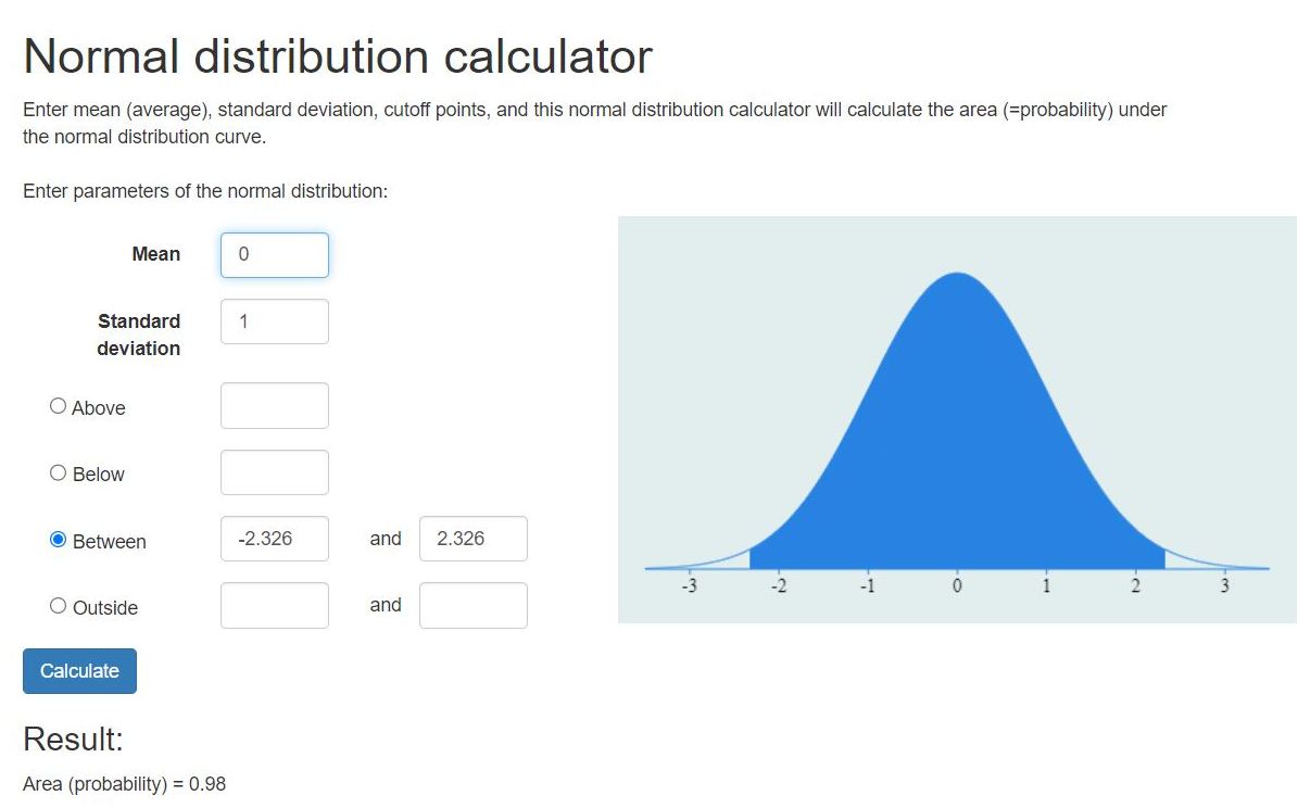
this is what it looks like using raw scores.
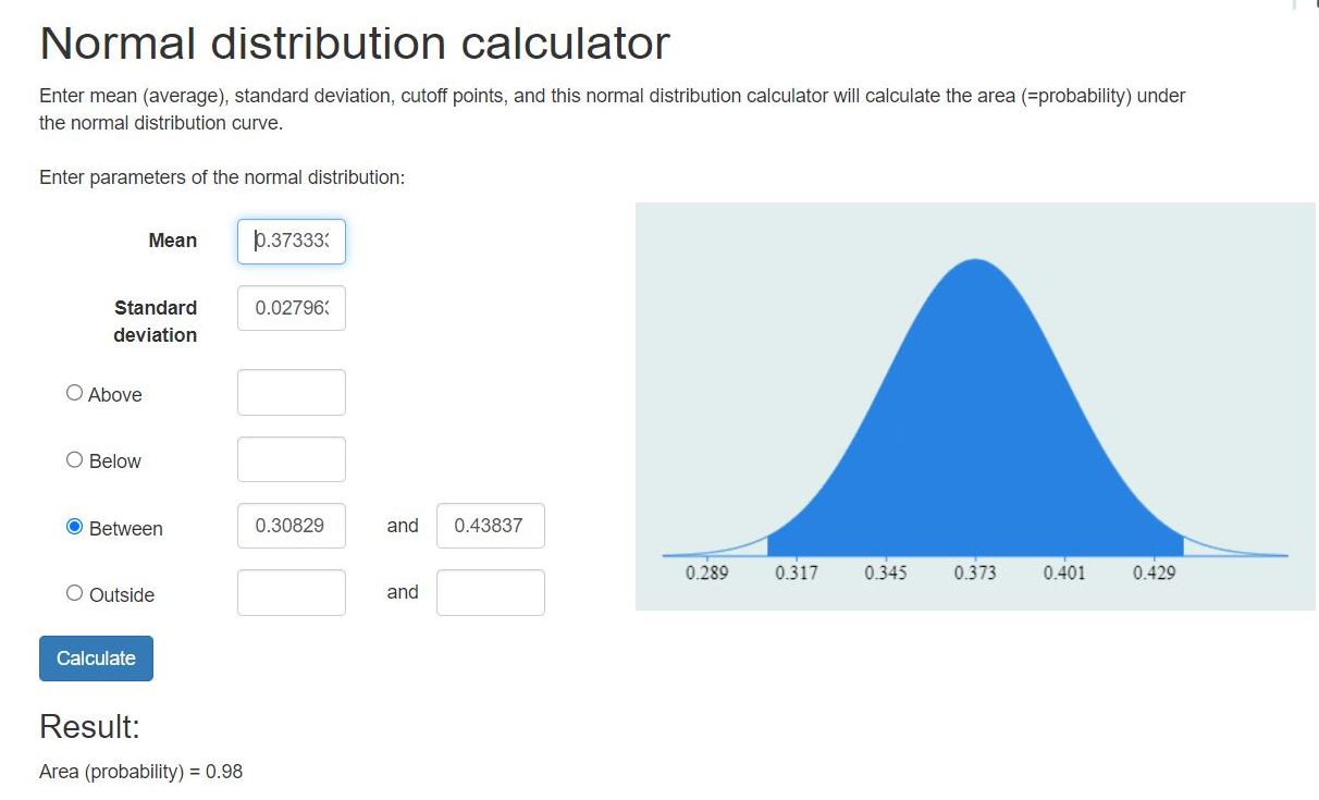
in the z-score formula:
z = the z-score
x = the sample proportion
m = the mean proportion which is equal to p
s = the standard error.
p is equal to the proportion of the sample size that favor an NDP candidate.
q = 1-p is equal to the proportion of the sample size that do not favor an NDP candidate.
the mean proportion is equal to p which is equal to m in the z-score formula.
Question 1205251: A quality controller of a company plans to inspect the average diameter of small bolts made. A random sample of 6 bolts was selected. The sample is computed to be 2.0016mm and the sample standard deviation 0.0012mm. Construct the 99% confidence interval for all bolts made.
Answer by Theo(13342) (Show Source):
You can put this solution on YOUR website! sample size is 6.
sample mean is 2.0016 millimeters.
sample standard deviation is .0012 millimeters.
since the sample mean and sample standard deviation are used, then the 99% confidence interval will be based on the t-score, rather than the z-score.
99% two tail confidence interval for t-score with 5 degrees of freedom (degrees of freedom equal sample size minus 1) is equal to t = plus or minus 4.032142983.
since you're looking at a distribution of sample means for samples of 6 elements each, the standard error is used.
standard error = standard deviation / sqrt(sample size) = .0012 / sqrt(6) = .0004898979486.
t-score formula is t = (x-m)/s
t is the critical t-score
x is the critical sample mean.
m is the sample mean.
s is the standard error.
on the low side of the confidence interval, the t-score formula becomes:
-4.032142983 = (x - 2.0016) / .0004898979486.
solve for x to get x = 1.999624661.
on the high side of the confidence interval, the t-score formula becomes:
4.032142983 = (x - 2.0016) / .0004898979486.
solve for x to get x = 2.003575339.
your two tail 99% confidence interval is from 1.999624661 to 2.003575339.
Question 1205253: A research firm conducted a survey to determine the mean amount smokers spend on cigarette during a week. A sample of 49 smokers revealed that the sample mean is Br. 20 with standard deviation of Br. 5. Construct 95% confidence interval for the mean amount spent.
Answer by math_tutor2020(3817) (Show Source):
You can put this solution on YOUR website!
At 95% confidence, the z critical value is roughly z = 1.96 which is something to memorize or have handy on a reference sheet somewhere.
n = 49 = sample size
xbar = 20 = sample mean
s = 5 = sample standard deviation
E = margin of error for the mean
E = z*s/sqrt(n)
E = 1.96*5/sqrt(49)
E = 1.4
L = lower boundary of the confidence interval
L = xbar - E
L = 20 - 1.4
L = 18.6
U = upper boundary of the confidence interval
U = xbar + E
U = 20 + 1.4
U = 21.4
The 95% confidence interval is approximately 18.6 < mu < 21.4
It's of the format L < mu < U.
We can condense that to the notation (18.6, 21.4)
Question 1205109: Ms. Lisa Monnin is the budget director for the New Process Company. She would like to compare the daily travel expenses for the sales staff and the audit staff. She collected the following sample information:
Sales ($)
131
135
146
165
136
142
Audit ($)
130
102
129
143
149
120
139
At the 0.10 significance level, can she conclude that the mean daily expenses are greater for the sales staff than the audit staff?
a. State the decision rule. (Round the final answer to 3 decimal places.)
Reject H0 if t >
1.363
.
b. Compute the pooled estimate of the population variance. (Round the final answer to 2 decimal places.)
Pooled estimate of the population variance
c. Compute the value of the test statistic. (Round the final answer to 3 decimal places.)
Value of the test statistic
d. State your decision about the null hypothesis.
Reject
H0 : μs ≤ μa.
e. Estimate the p-value. (Round the final answer to 4 decimal places.)
The p-value is
.
Answer by Theo(13342) (Show Source):
You can put this solution on YOUR website! this looks like a two sample t-test.
there is a calculator that provides that analysis online.
the calculator can be found at https://www.statskingdom.com/140MeanT2eq.html
the results of that analysis are shown below.
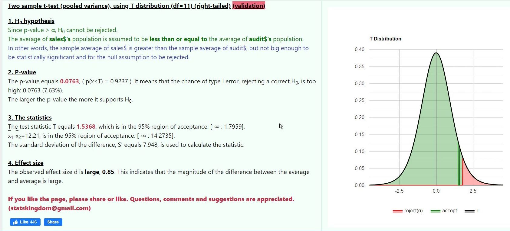
the p-value of the test was .0763 which was less than the critical p-value of .10.
the test was a one tail test on the high side of the confidence interval because the criteria was to see if sales group mean was greater than audit group mean.
this placed the critical alpha all on the right side of the confidence interval.
the calculator calculated the mean of each sample and the variance of each sample.
the variances from both samples were then pooled to provide a common variance that was then used to calculate the standard error of the test.
a reference for pooled variance calculations is shown below.
https://stats.libretexts.org/Bookshelves/Applied_Statistics/Natural_Resources_Biometrics_(Kiernan)/04%3A_Inferences_about_the_Differences_of_Two_Populations/4.02%3A_Pooled_Two-sampled_t-test_(Assuming_Equal_Variances)#:~:text=Pooling%20refers%20to%20finding%20a,of%20the%20two%20sample%20variances.&text=If%20n1%3Dn2,of%20the%20two%20sample%20variances.
i calculated the pooled variance manually and then calculated the standard error based on that reference and it agreed with the results of the calculator.
i also calculated the mean of each sample and the standard deviation of each ample and they also agreed with what the calculator showed.
my calculations showed the the mean of the sale data was 142.5 and the mean of the mean of the audit data was 130.285 (rounded results, not full detail).
my calculations also showed that the standard error was 7.94789.
i used those values to calculate the t-score with 11 degrees of freedom and got the following.
t = (142.5 - 130.285) / 7.94789 = 1.53688.
that was close enough for me to determine that the manual results and the calculator results were consistent with each other.
the pooled variance was equal to 5 * (12.24336)^2 + 6 * (15.787276)^2 / 11 = 204.084415.
the standard error was equal to the square root of that * sqrt(1/6 + 1/7) = 7.94789.
i also calculated the standard deviation of each sample using my ti-84 plus calculator..
it was 12.243365 for sale date an 15.787276 for audit data.
the variance for each would be the square of that.
bottom line:
the results were not significant indicating there was insufficient evidence to make the conclusion that mean of sales data was higher than mean of audit data.
let me know if you have any questions.
theo
Question 1202346: sketch the rejection region for a one-tailed test with 90% confidence.
Does z = 1.84, fall in the rejection
region
Answer by Theo(13342) (Show Source):
You can put this solution on YOUR website! see the following graph.
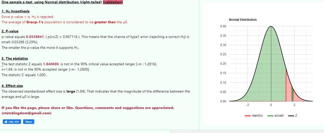
the tst z-score was 1.84.
the critical z-score at 90% right tailed confidence interval qas 1.28.
since the test z-scorre was grater than the critical z-score, it ws in the rejection region, as shown on the graph.
Question 1201813: In a study of 420,113 cell phone users, 136 subjects developed cancer of the brain or nervous system. Test the claim of a somewhat common belief that such cancers are affected by cell phone use. That is, test the claim that cell phone users develop cancer of the brain or nervous system at a rate that is different from the rate of 0.0340% for people who do not use cell phones. Because this issue has such great importance, use a 0.001significance level. Identify the null hypothesis, alternative hypothesis, test statistic, P-value, conclusion about the null hypothesis, and final conclusion that addresses the original claim. Use the P-value method and the normal distribution as an approximation to the binomial distribution.
Answer by Theo(13342) (Show Source):
You can put this solution on YOUR website! 420,113 cell phone users.
136 developed cancer of the brain or nervous system.
sample p = 136 / 420,113 = .0003237224271.
population p assumed to be .034% / 100 = .00034.
standard error = sqrt (p * q / n) = sqrt (,99923 * (1 - .00034) / 420113) = .00002844346856.
test z-score = (sample mean minus assumed population mean) divided by standard error = (.0003237224271 - .00034) / .00002844346856 = -.5722780576.
area to the left of that = .2835667641.
that's greater than the critical p-value of .0005 (two tailed critical alpha is .001 / 2 = .0005 on each end), so the results are not considered significant.
the critical z-score on the low end was equal to -3.290526729.
the test z-score was considerably less than that, reinforcing the p-value concluson of no significance.
Question 1200133: -An experimental surgical procedure is being studied as an alternative to the existing method. Twelve surgeons perform the operation on two different patients matched by sex, age and other relevant factors.
Problem Definition: Determine whether or not the new procedure is faster than the existing procedure. Alpha is .05
I NEED HELP WITH THIS STEP BELOW. I PUT ALL THE DATA INTO MINITAB AND CAME UP WITH THE STATISTICS BUT I'M NOT SURE BOW TO INTERPRET IT:
-Utilize all three techniches: critical value technique, the confidence interval and the p-value in your conclusion. Include the numbers from the minitab output for each technique. Write your assumption and discuss how you know whether or not normality may be assumed.
Descriptive Statistics:
Sample N Mean StDev SE Mean
New Procedure 12 13.25 2.38 0.69
Old Procedure 12 23.42 3.58 1.03
Estimation for Paired Difference:
Mean StDev SE Mean 95% Upper Bound
for μ_difference
-10.17 3.83 1.11 -8.18
µ_difference: population mean of (New Procedure - Old Procedure)
Test:
Null hypothesis H₀: μ_difference = 0
Alternative hypothesis H₁: μ_difference < 0
T-Value P-Value
-9.19 0.000
Answer by math_tutor2020(3817) (Show Source):
You can put this solution on YOUR website!
The Minitab output you copy/pasted doesn't appear to be fully coherent.
The critical value and confidence interval information is either missing, or garbled in the table.
However, the p-value appears to be intact.
A p-value of 0.000 means it's so small that it's practically zero.
Since the p-value is smaller than alpha = 0.05, we reject the null. A handy phrase could be "If the p-value is low, then the null must go".
So we go with
Alternative hypothesis H1: μ_difference < 0
and conclude that the new experimental surgical procedure appears to be faster than the existing procedure.
Question 1200159: A school conducts an interest aptitude test for final students, the teacher think that the average student aptitude test score is 470 with a known standard deviation value of 10, so the school takes a sample of the talent interest test value data from 9 students as follows:
Student A Score 440
Student B Score 460
Student C Score 485
Student D Score 509
Student E Score 496
Student F Score 477
Student G Score 457
Student H Score 465
Student I Score 495
The hypothesis put forward by the management department is as follows:
H0: μ = 470
H1: μ # 470
By using a = 5%, testing in two tails (two sides), test this opinion and give the conclusion!
Note:
Do this problem using manual formulas in a structured manner, don't use calculations from excel, minitab, or the like.
Answer by math_tutor2020(3817) (Show Source):
You can put this solution on YOUR website!
Given information:
mu = 470 = mean
sigma = 10 = standard deviation
Data set = {440, 460, 485, 509, 496, 477, 457, 465, 495}
n = 9 = sample size
alpha = 0.05 = significance level
Hypotheses:
H0: μ = 470
H1: μ # 470
This is a two tailed test due to the "not equal" sign in the alternative hypothesis.
Let's calculate the sample mean xbar.
xbar = (sum of the scores)/(sample size)
xbar = (440+460+485+509+496+477+457+465+495)/(9)
xbar = (4284)/(9)
xbar = 476
Compute the test statistic
z = (xbar - mu)/(sigma/sqrt(n))
z = (476 - 470)/(10/sqrt(9))
z = 1.8
Take notice how I'm using the Z distribution instead of T distribution.
This is because the value of sigma is known.
Use a Z table like this one
https://www.ztable.net/
such tables are found in the back of your stats textbook.
For exams, your teacher would likely give you a reference sheet.
Use that table to find that
P(Z < 1.80) = 0.96407
This value is found in the row that starts with +1.8, and it is in the column that has 0 at the very top.
Scroll down to the section titled "How to Read The Z Table" on that page for more information and an example.
Since P(Z < 1.80) = 0.96407, this means the area to the left of z = 1.80 is roughly 0.96407
The area to the right of this z score is...
P(Z > 1.80) = 1 - P(Z < 1.80)
P(Z > 1.80) = 1 - 0.96407
P(Z > 1.80) = 0.03593
We double this value since we're doing a two tailed test.
0.03593 doubles to 0.07186 which is the approximate p-value.
Rule: if the p-value is smaller than alpha, then reject the null.
We have
alpha = 0.05
p-value = 0.07186
and can see that the p-value is not smaller than alpha, so we fail to reject the null. This means we have no choice but to "accept" the null until more information comes along to disprove it.
Conclusion: Accept the null hypothesis that μ = 470 is the case.
Interpretation: The mean test score appears to be 470. The teacher's claim appears to be correct.
Question 1198408: A researcher claims that 15% of children suffer from chronic ear infections. A sample of 100 children was taken and it was found that 18% of the children suffer from chronic ear infections. Test at the 1% significance level if the proportion of children that suffer from a chronic ear infection is different from 15%. What is the p-value?
Answer by ewatrrr(24785)  (Show Source): (Show Source):
You can put this solution on YOUR website! Ho: p = .15
Ha: p ≠ .15
two-tailed
Sample: n = 100, x̄ = .18,
.01 significance level
z =  = -.84 = -.84
p = .2
.2 > .01, Fail to reject Ho.
Evidence not sufficient to support p ≠ .15
Question 1197931: Arnold Palmer and Tiger Woods are two of the best golfers to ever play the game. To show how these two golfers would compare if both were playing at the top of their game, the following sample data provide the results of 18-hole scores during a PGA tournament competition. Palmer’s scores are from his 1960 season, while Woods’s scores are from his 1999 season (Golf Magazine, February 2000).
Palmer, 1960 Woods, 1999
n_1 = 112 n_2 = 84
x_1 = 69.95 x_2 = 69.56
Use the sample results to test the hypothesis of no difference between the population mean 18-hole scores for the two golfers.
a. Assume a population standard deviation of 2.5 for both golfers. What is the value of the test statistic?
b. What is the p-value?
c. At α = .01, what is your conclusion?
Answer by ewatrrr(24785) (Show Source):
You can put this solution on YOUR website! Ho: m1 - m2 = 0
Ha: m1 - m2 > 0
α = .01
t=(x̄1 - x̄2)/sqrt ((s1^2/n1)+(s2^2/n2))
t=(69.95-69.56)/sqrt ((2.5/112)+(2.5/84)) = 1.71
p(z > 1.71) = .0436 > .01 , Fail to reject Ho.
Sample results indicate there is no difference between the population mean 18-hole scores for the two golfers.
Question 1196805: Calculate the p-value of the test to determine that there is sufficient evidence to infer each research objective.
Research objective: The population mean is greater than 0.
σ=10, n=100, x-bar= 1.5
Answer by ewatrrr(24785) (Show Source):
You can put this solution on YOUR website!
Hi
Calculate the p-value of the test to determine that there is sufficient evidence to infer u > 0

n= 100,  x̄ = 1.5
Ho: u ≤ 0        Note:  Ho MUST contain equality:: = or ≤ or  ≥
Ha: u > 0  claim
generally a 95% confidence level is used.  alpha = 0.05

  = 1.5
    p(1.5) = normalpdf(1.5)= .13   Using Calculator
  .13 > .05  Fail to Reject Ho
(Note:  If the p-value is greater than alpha = 0.05, so we fail to reject the null hypothesis)
That is: There is NOT sufficient evidence, at the 0.05 level of significance, to support a claim that u > 0 = 1.5
p(1.5) = normalpdf(1.5)= .13 Using Calculator
.13 > .05 Fail to Reject Ho
(Note: If the p-value is greater than alpha = 0.05, so we fail to reject the null hypothesis)
That is: There is NOT sufficient evidence, at the 0.05 level of significance, to support a claim that u > 0
Question 1196806: Calculate the p-value of the test to determine that there is sufficient evidence to infer each research objective.
Research objective: The population mean is greater than 0.
σ=10, n=100, x-bar= 1.5
Answer by Theo(13342) (Show Source):
You can put this solution on YOUR website! the research objective is that the population mean is greater than 0.
the null assumption is therefore that the population mean is not greater than 0.
the sample mean is 1.5
the sample size = 100
the sample standard deviation is 10
the standard error = standard deviation / sqrt(sample size) = 10/10 = 1
t-score = (x - m) / s = (1.5 - 0) / 1 = 1.5
p-value to the right of this t-score at 99 degrees of freedom (sample size - 1) = .064.
the results are not significant at right tailed alpha of .05 because the test alpha is greater than that.
alternate hypothesis that population mean is greater than 1.5 is therefore rejected.
the results from the t-test calculator at https://www.statskingdom.com/130MeanT1.html confirm this.
see below:
Question 1195831: A study was conducted to determine weight loss, body composition, etc. in obese women before and after 12 weeks of treatment with a very-low-calorie diet: (05 Marks)
Before After
85 86
95 90
75 72
110 100
81 75
92 88
83 83
94 93
88 82
105 99
We wish to know if these data provide sufficient evidence to allow us to conclude that the treatment is effective in causing weight reduction in obese women at . Solve using five step critical - value approach.
Answer by Boreal(15235)  (Show Source): (Show Source):
You can put this solution on YOUR website! Ho: Change is 0
Ha: Change is not 0
alpha=0.05 p{reject Ho|Ho true}
test is a paired t (0.975, df=9) critical value |t| > 2.262
values
mean is 4
s=3.33
t=difference/s/sqrt(n)
=4/3.333/sqrt(10)
=3.798
Reject Ho; the mean difference is positive, not 0, and there is a significant difference in the treatment to cause weight loss. p-value=0.004.
Question 1194813: Some manufacturers claim that non-hybrid sedan cars have a lower mean miles-per-gallon (mpg) than hybrid ones. Suppose that consumers test 21 hybrid sedans and get a mean of 31 mpg with a standard deviation of seven mpg. 18non-hybrid sedans get a mean of 22 mpg with a standard deviation of four mpg. At 0.05 level of significance, conduct a hypothesis test to evaluate the manufacturers claim.
Answer by Boreal(15235) (Show Source):
You can put this solution on YOUR website! Ho: NH>= H
Ha: NH< H
alpha=0.05 p{reject Ho|Ho true}
test statistic is a t (0.95, df=37)
critical value is t < -1.687
t=(NH-H)/sqrt (sH^2/n1)+(sNH^2/n2)
=-9/sqrt((49/21)+(16/18))
=-9/1.80
=-5
strongly reject Ho and conclude that the manufacturer's claim is correct.
p <0.0001
Question 1194538: The profits of a corner store for 6 days are 2,000 pesos, 3,000 pesos, 1,200 pesos, 6,000 pesos,
4,000 pesos, and 5,100 pesos. Does this set of data present sufficient evidence that the average
profit per day of the store is more than 3,800 pesos per day? Test at the 0.05 level of
significance.
Answer by Boreal(15235) (Show Source):
You can put this solution on YOUR website! this is a one sample t-test
Ho: mean is <= 3800
Ha:: mean is >3800
alpha=0.05 p{reject Ho|Ho true}
test is t (0.95, df=5)
critical value t>2.015
t=(x bar-mean)/s/sqrt(n)
=(3550-3800)/1835/sqrt(6)
=-250*sqrt(6)/1835
=-0.333
fail to reject Ho (obvious, since mean of sample- hypothesized mean is < 0.
Question 1193394: 1.The mean number of close friends for the population of people living in the Philippines is 5. The standard deviation of scores in this population is 1.2. An investigator predicts that the mean number of close friends for intorverts will be significantly different from the mean of the population. The mean number of close friends for a sample of 26 introverts is 6. Find the z-value *
Answer by Boreal(15235) (Show Source):
Question 1192845: Ocho Rios Autoworks, a chain of automotive tune-up shops, advertises that its personnel can change oil, replace the oil filter, and lubricate any standard automobile in 15minutes, on the average. The Bureau of Standards received complaints from customers that service
takes considerably longer. To check the firm's claim, the Bureau had service done on 21 unmarked cars. The mean service time was 17 minutes, and the standard deviation of the sample was 1 minute. Use the 0.05 level of significance to check the reasonableness of the
claim made by Ocho Rios Autoworks.
Z = (X - U) / (SD / √n)
=17-15/1/sqrt(21)
= 9.165
I have never gotten a z value so large before, please advise if I am doing something wrong
Answer by Theo(13342) (Show Source):
You can put this solution on YOUR website! you did it right.
it is very possible to get z-score that are very high or very low.
this is one example of that.
it can get even higher than that.
assuming the average time was 30 minutes with a standard deviation of 1 minute and a sample size of 21, then the z-score could have been (30 - 15) / (1/sqrt(21)) = 68.7...
it all depends on what the actual wait time was versus what the claimed wait time was.
Question 1192252: In a 1868 paper, German physician Carl Wunderlich reported based on over a million body temperature readings that the mean body temperature for healthy adults is 98.6° F. However, it is now commonly believed that the mean body temperature of a healthy adult is less than what was reported in that paper. To test this hypothesis a researcher measures the following body temperatures from a random sample of healthy adults.
98.2, 98.5, 98.6, 98.5, 97.3, 98.3
(a) Find the value of the test statistic.
Answer by Boreal(15235) (Show Source):
Question 1192085: The contents of 33 cans of Coke have a sample mean of x =12.15 and a standard deviation of s=0.11. Find the value of the test statistic t for the claim that the population mean is μ=12.
Answer by Theo(13342) (Show Source):
You can put this solution on YOUR website! n = 33
sample mean = 12.15
sample standard deviation = .11
claim is population mean is 12
standard error = sample standard deviation / square root of sample size = .11/sqrt(33) = .01915.
t-score = (x - m) / s = (sample mean minus assumed mean) / standard error = (12.15 - 12) / .01915 = 7.83.
that would be the test statistic.
Question 1187490: The Mathematical Anxiety Rating Scale (MARS) measures an individuals level of mathematical anxiety on a scale from 25 (no anxiety) to 100 (highest anxiety). A group of researcher administered the MARS to 50 students. One of the objectives of the study was to determine if there is a difference between levels of mathematical anxiety experienced by male and female psychology students.
alpha level=0.05level of significance, is there evidence of a difference in the mean mathematical anxiety experienced by male and female psychology students?
Solution:
Step 1: State the hypotheses
Ho:
Ha:
Step 2: The level of significance and the critical region
Step 3: Compute for the value of t test.
Step 4: Decision rule.
Step 5. Conclusion.
Please help me with this problem, this is the only problem that I haven't finished yet 🥺 and the deadline will be this coming Wednesday. Thankyou in advance. GB
Nov. 10 11:59 pm
Answer by Boreal(15235) (Show Source):
You can put this solution on YOUR website! let M be the mean of the male students; F the mean of the female students.
Ho: M=F
Ha:M NE F;they are unequal
alpha=0.05 p{reject Ho|Ho true}
test statistic is a t(0.975, df=48)
critical value can be looked up for that test statistic. Reject if |t| > 2.01
Compute the value where t=(M-F)/sqrt ((sdM^2/25)+(sdF^2/25)
or get the pooled variance and the denominator is sp * sqrt ((1/n1)+(1/n2)). Some use it, others don't.
Compare with critical value.
Reject the null hypothesis; the two are different OR fail to reject the null hypothesis, insufficient evidence to say the two are different.
Question 1184842: What are the Z values at 0.10 significance level.
Answer by Edwin McCravy(20055)  (Show Source): (Show Source):
You can put this solution on YOUR website!
That depends on whether you are using a 1-tail test or a 2-tail test.

If it's a 1-tail test, it's the z-value that has the entire area of 0.10 to
the right of it, and therefore it has an area of 0.95 before it.

On your T-84

Press 2ND VARS 3

Make the screen read

area:0.95
μ:0
σ:1
Paste

Use down arrow key to scroll to highlight Paste

Press ENTER

Read

invNorm(0.95,0,1)

Press ENTER

Read 1.644853626 round as your teach said, probably to 1.645

--------------------------

If it's a 2 tail test, it's the z value that has area of one-half of 0.10 to
the right of it, and therefore it has an area of 0.90 before it.

On your T-84

Press 2ND VARS 3

Make the screen read

area:0.90
μ:0
σ:1
Paste

Use down arrow key to scroll to highlight Paste

Press ENTER

Read

invNorm(0.90,0,1)

Press ENTER

Read 1.281551567 round as your teacher said, probably to 1.28

Edwin
Question 1183969: It has been determined that 37 out of 100 adult Americans that did not attend college believe in extra-terrestrials. However, from a random sample of 100 adult Americans that did not attend college 43 claim that they believe in extra-terrestrials. Does this indicate that the proportion of people who did not attend college and who believe in extra-terrestrials has changed? Conduct a hypothesis test with a = 0.01 and interpret the results. (10 points)
Answer by Boreal(15235) (Show Source):
You can put this solution on YOUR website! Ho: proportion =0.43
Ha: proportion NE 0.43
alpha=0.01 p{reject Ho|Ho true}
test is a z
reject for |z|>2.576
calculate z=(phat-p)/sqrt(0.37*0.63/100)
=0.06/0.048
=1.24
fail to reject Ho; insufficient evidence to say there is a difference at the 1% level of significance.
p-value=0.22
Question 1183752: For each of the following tobs values, determine the highest level of
significance associated with the decision taken.
tobs df Decision
(i) 4.000 17 Reject Ha for a two-tailed test
(ii) 1.200 120 Reject Ha for a one-tailed test
(iii) -2.660 16 Reject Ha for both one-tailed
and two-tailed test
(iv) -1.586 60 Reject Ha for a one-tailed te
Answer by MathLover1(20849)  (Show Source): (Show Source):
Question 1183210:
Answer by ikleyn(52781)  (Show Source): (Show Source):
Question 1183211:
Answer by ikleyn(52781) (Show Source):
Question 1181946: The ABM Coffee Company claims that 20% of the coffee drinkers in Pinalagad, Malinta prefer their brand, the Ang Barako Mo coffee. To test the claim, a group of CNHS Grade 11 students conducted a survey, which they found out. Out of the 500 randomly selected residents, 95 indicated that ABM coffee is the reason why they wake up in the morning. Set up the Rejection Region and the Critical Values for Left-Tailed, Right-Tailed, and Two-Tailed tests. Use ɑ=.10.
Answer by Boreal(15235) (Show Source):
You can put this solution on YOUR website! Ho: ABM has 20% preference
Ha: ABM does not have 20% preference (2-tailed) and critical value |z|>1.645.
-
Ho: ABM has less than or =20% preference
Ha: ABM has > 20% preference (right-tail) with critical value z>1.282
-
Ho: ABM has greater than or equal to 20% preference.
Ha: ABM has < 20% preference (left-tail) with critical value z < -1.282
-
I learned hypothesis tests in that both have to cover the entire possibility, and that generally equal goes with the null hypothesis.
Also, the direction of the data should be noted. Here, the percentage is 19%, so one would expect the alternative hypothesis to be < 20% OR not equal to 20%. If the alternative hypothesis is greater than 20%, the data don't show it a priori.
-
The equation is z=(p hat-p)/sqrt(0.2*0.8/500)
=-0.01/sqrt(.16/500)
=-0.559
|
|