Questions on Algebra: Probability and statistics answered by real tutors!

Tutors Answer Your Questions about Probability-and-statistics (FREE)

Question 1164546: a) Plot the pmf and cdf of the geometric random variable X with probability of success p = 1/3.
b) Find E[X] and var(X).
c) Find P(X > 4)
Found 3 solutions by MathTherapy, mccravyedwin, amarjeeth123:
Answer by MathTherapy(10806)   (Show Source):
You can put this solution on YOUR website!

It’s good to see you again, Sir Edwin! Haven’t seen you in a while. How are you? Are you okay? Had you grown tired of this author and others in this forum, and decided to take a break? Amyway, welcome back!

Answer by mccravyedwin(421)   (Show Source):
You can put this solution on YOUR website!

This concerns getting the probablity that we will get our first success on the kth trial, with a probability of success on each trial being p = 1/3. The other tutor was correct for part b), which was: b) a) Instead of plotting, I'll just list the values: PMF(probability mass function) CDF(cumulative distribution function) k|PMF(k) |CDF(k) 1|0.3333 |0.3333 2|0.2222 |0.5556 3|0.1481 |0.7037 4|0.0988 |0.8025 5|0.0658 |0.8683 6|0.0439 |0.9122 7|0.0293 |0.9415 8|0.0195 |0.9610 9|0.0130 |0.9740 10|0.0087 |0.9827 c) (approximately) Edwin

Answer by amarjeeth123(574)   (Show Source):
You can put this solution on YOUR website!
E[X]=1/p=1/(1/3)=3
Var[X]=((1-p)/p^2)=(2/3)/(1/9)=(2/3)*9=2*3=6
Since the number of trials is not given we cannot calculate the desired probability.

Question 1158881: Suppose that 69 of all college seniors have a job prior to graduation. If a random sample of 50 college seniors is taken, approximate the probability that more than 37 have a job prior to graduation. Use the normal approximation to the binomial with a correction for continuity.
Round your answer to at least three decimal places. Do not round any intermediate steps.
Answer by ikleyn(53748)   (Show Source):
You can put this solution on YOUR website!
.

Was solved at this forum under this link

https://www.algebra.com/algebra/homework/Probability-and-statistics/Probability-and-statistics.faq.question.1159211.html

Question 1164737: A trading company has eight computers that it uses to trade on the New York Stock Exchange
(NYSE). The probability of a computer failing in a day is 0.005, and the computers fail
independently. Computers are repaired in the evening and each day is an independent trial.
(a) What is the probability that all eight computers fail in a day?
(b) What is the mean number of days until a specific computer fails?
(c) What is the mean number of days until all eight computers fail in the same day
compute the solution in R ?
Found 2 solutions by ikleyn, CPhill:
Answer by ikleyn(53748)   (Show Source):
You can put this solution on YOUR website!
.
A trading company has eight computers that it uses to trade on the New York Stock Exchange
(NYSE). The probability of a computer failing in a day is 0.005, and the computers fail
independently. Computers are repaired in the evening and each day is an independent trial.
(a) What is the probability that all eight computers fail in a day?
(b) What is the mean number of days until a specific computer fails?
(c) What is the mean number of days until all eight computers fail in the same day
compute the solution in R ?
~~~~~~~~~~~~~~~~~~~~~~~~~~~~~~~

(a) What is the probability that all eight computers fail in a day? This probability is P = = 3.90625E-19. ANSWER Interesting to note that this number is a PRECISE value - not an approximate ! (b) What is the mean number of days until a specific computer fails? The mean number of days until a specific computer fails is = 200 days. ANSWER (c) What is the mean number of days until all eight computers fail in the same day The mean number of days until all eight computers fail in the same day is = 2.56E+18 = days. ANSWER According to the current knowledge, our Universe exists about 13.8 billion years, which is less than the answer to this question.

Solved. All questions are answered.

Answer by CPhill(2189)   (Show Source):
You can put this solution on YOUR website!
To solve this, we will use the properties of the **Binomial Distribution** (for successes in a fixed number of trials) and the **Geometric Distribution** (for the time until an event occurs).
### Mathematical Breakdown
**Part (a): Probability that all eight computers fail in a day**
Since each computer is an independent trial with a constant probability of failure , the number of failures follows a Binomial distribution: .
The probability of all 8 failing is:

**Part (b): Mean number of days until a specific computer fails**
The number of days until a specific event occurs follows a Geometric distribution. The mean (expected value) is given by:

**Part (c): Mean number of days until all eight computers fail on the same day**
In this case, we treat the "event" as the simultaneous failure of all 8 computers. Let the probability found in part (a) be . The mean number of days until this specific event occurs is:

---
### R Solution
You can copy and paste the following code into your R console or RStudio:
```r
# Define parameters
n <- 8
p <- 0.005
# (a) Probability that all eight computers fail in a day
# Using the dbinom function or direct calculation
prob_all_fail <- dbinom(8, size = n, prob = p)
# prob_all_fail <- p^8
cat("(a) Probability all 8 fail in a day:", format(prob_all_fail, scientific = TRUE), "\n")
# (b) Mean number of days until a specific computer fails
# Mean of Geometric distribution is 1/p
mean_days_specific <- 1 / p
cat("(b) Mean days until a specific computer fails:", mean_days_specific, "days\n")
# (c) Mean number of days until all eight computers fail in the same day
# Mean is 1 over the probability of the event occurring
mean_days_all_fail <- 1 / prob_all_fail
cat("(c) Mean days until all 8 fail on same day:", format(mean_days_all_fail, big.mark = ","), "days\n")
```
### Explanation of Results
* **(a)** The probability is . This is effectively zero, making it an extremely rare "black swan" event.
* **(b)** On average, you can expect a specific computer to fail once every **200 days**.
* **(c)** The mean wait time for all 8 to fail at once is ** days**. For perspective, the universe is approximately days old, so this event is statistically unlikely to ever happen in human history.
Would you like to see how the probability changes if the computers were not independent (e.g., a power surge affecting all of them at once)?

Question 1164684: In order to manage the Credit Risk, a bank regularly rates each of its borrowers as Al or A2 or A3, based on their Credit history. A1 implies lowest risk and A3 implies highest risk. Risk means the chance that a borrower might fail to pay back the loan amounts. Based on historical data, on an average, 30% customers are rated Al, 60% are rated A2, and 10% are rated A3. It was found that 1% of the customers who were rated Al, 10% of the customers who were rated A2, and 18% of the customers who were rated A3, eventually became defaulters (failed to payback). If you randomly pick up a customer from defaulter's pool, what is the probability that he had received an Al rating?
Answer by ikleyn(53748)   (Show Source):
You can put this solution on YOUR website!
.
In order to manage the Credit Risk, a bank regularly rates each of its borrowers as Al or A2 or A3, based on their Credit
history. A1 implies lowest risk and A3 implies highest risk. Risk means the chance that a borrower might fail to pay back
the loan amounts. Based on historical data, on an average, 30% customers are rated Al, 60% are rated A2, and 10% are rated
A3. It was found that 1% of the customers who were rated Al, 10% of the customers who were rated A2, and 18% of the
customers who were rated A3, eventually became defaulters (failed to payback). If you randomly pick up a customer from
defaulter's pool, what is the probability that he had received an Al rating?
~~~~~~~~~~~~~~~~~~~~~~~~~~~~

This probability is P = 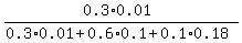= 0.37. +---------------------------------------------------+ | It is important to understand | | the structure and the meaning of this formula. | +---------------------------------------------------+ Its denominator is the probability for a randomly pick up customer to be in the defaulters' pool. Its numerator is the probability for a randomly pick up customer to satisfy two conditions: (a) to be in section A1 AND (at the same time) (b) to be in the defaulters' pool. The formula in whole is the standard formula for the conditional probability.

Solved and explained completely.

----------------------------

Now, as you know this formula, its structure and meaning, you can solve
many other similar conditional probability problems on your own.

My post is a standard mantra to pronounce while solving such problems.

Happy learning !

Come again to this forum soon to learn something new !

Question 1164707: Five observations have been drawn independently and at random from
a continuous distribution. What is the probability that the next observation
will be less than all of the first five?
Found 2 solutions by greenestamps, CPhill:
Answer by greenestamps(13327)   (Show Source):
You can put this solution on YOUR website!

The problem is equivalent to this:

Make 6 observations and list them in order from least to greatest. What is the probability that the 6th observation is first in the list?

Using the basic definition of probability, there are 6 possibilities for which one of the 6 observations is first; there is only one possibility for the 6th observation to be first; so the probability that the 6th observation is first in the list is 1/6.

ANSWER: 1/6

Answer by CPhill(2189)   (Show Source):
You can put this solution on YOUR website!
This is a classic problem in **non-parametric statistics** and **symmetry**. Because the observations are drawn from a continuous distribution, the probability that any two observations are exactly equal is zero.
### The Symmetry Argument
When you have a set of independent and identically distributed (i.i.d.) random variables, every possible ordering of those variables is **equally likely**.
1. Let the first five observations be .
2. Let the next observation be .
3. We now have a total of **6 observations** in our set.
In a set of 6 independent observations from the same continuous distribution, any one of them is just as likely to be the "minimum" as any other.
### Calculation
Since there are 6 observations and each has an equal chance of being the smallest value:
* The probability that is the smallest is .
* The probability that is the smallest is .
* ...and so on.
The probability that the **next observation ()** is the smallest (less than all of the first five) is:

**The probability is 1/6 (or approximately 0.1667).**
---
### Key Intuition
It does not matter what the actual distribution is (Normal, Uniform, Exponential, etc.). As long as the observations are independent and come from the same continuous distribution, the "rank" of the sixth observation is distributed uniformly among the possibilities .
Would you like to see how this probability changes if we were looking for the probability that the sixth observation is the *median* instead of the *minimum*?

Question 1164818: A lot of 75 washers contains 5 in which the variability in thickness around the circumference
of the washer is unacceptable. A sample of 10 washers is selected at random, without
replacement.
(a) What is the probability that none of the unacceptable washers is in the sample?
(b) What is the probability that at least one unacceptable washer is in the sample?
(c) What is the probability that exactly one unacceptable washer is in the sample?
(d) What is the mean number of unacceptable washers in the sample?

Also give R code
Found 2 solutions by ikleyn, CPhill:
Answer by ikleyn(53748)   (Show Source):
You can put this solution on YOUR website!
.
A lot of 75 washers contains 5 in which the variability in thickness around the circumference
of the washer is unacceptable. A sample of 10 washers is selected at random, without
replacement.
(a) What is the probability that none of the unacceptable washers is in the sample?
(b) What is the probability that at least one unacceptable washer is in the sample?
(c) What is the probability that exactly one unacceptable washer is in the sample?
(d) What is the mean number of unacceptable washers in the sample?
~~~~~~~~~~~~~~~~~~~~~~~~~~

(a) What is the probability that none of the unacceptable washers is in the sample? One way to calculate is to use the formula P = = . The numerator is the number of favorable choices from 70 good washers taken 5 at a time; the denominator is the number of all possible choices from 75 washers taken 5 at a time. This is the ratio of two very big numbers (12-digits or 11-digits). They can be calculated in the scientific format, but this way does not give the feeling of numbers. So, I prefer another (equivalent) formula P = = 0.4786 (rounded). ANSWER This formula is self-explanatory. Part (a) is solved. (b) What is the probability that at least one unacceptable washer is in the sample? This probability is the complement P' = 1 - P = 1 - 0.4786 = 0.5214 (rounded). ANSWER Part (b) is solved. (c) What is the probability that exactly one unacceptable washer is in the sample? One way to calculate is to use the formula P = . Again, this is the ratio of two very big numbers (12-digits or 11-digits). They can be calculated in the scientific format, but this way does not give the feeling of numbers. So, I prefer another (equivalent) formula P = = 0.5178 (rounded). ANSWER Part (c) is solved. (d) What is the mean number of unacceptable washers in the sample? It is = .

Solved. All questions are answered.

/\/\/\/\/\/\/\/\/\/\/\/\/\/\/\/

I submit this my solution as an opposition to the post by @CPhill.

I want you see the difference between a true Math solution,
which teaches on how to solve a typical Math problem by a traditional way and how to makes it effectively
in opposite to the post by @CPhill, which is the run of the undebugged computer code
and demonstrates how the Artificial Intelligence should not communicate with a user.

Answer by CPhill(2189)   (Show Source):
You can put this solution on YOUR website!
Since the sample is selected **without replacement** from a finite population, this problem follows a **Hypergeometric Distribution**.
### Given Parameters:
* **Total population size ():** 75 washers
* **Number of successes in population ():** 5 unacceptable washers
* **Number of failures in population ():** 70 acceptable washers
* **Sample size ():** 10 washers
The probability mass function for the hypergeometric distribution is:

---
### (a) Probability that none of the unacceptable washers is in the sample
We are looking for . This means we choose 0 from the 5 unacceptable and 10 from the 70 acceptable washers.

Calculating this:

---
### (b) Probability that at least one unacceptable washer is in the sample
This is the complement of "none are unacceptable":

---
### (c) Probability that exactly one unacceptable washer is in the sample
We are looking for . This means we choose 1 from the 5 unacceptable and 9 from the 70 acceptable washers.

Calculating this:

---
### (d) Mean number of unacceptable washers in the sample
For a hypergeometric distribution, the mean is calculated as:

---
### R Code
You can use the built-in `dhyper` (for exact probability) and `phyper` (for cumulative probability) functions in R.
```r
# Parameters
N <- 75 # Total population
K <- 5 # Unacceptable in population
n <- 10 # Sample size
m <- K # Number of 'success' items (unacceptable)
nn <- N - K # Number of 'failure' items (acceptable)
# (a) Probability X = 0
prob_a <- dhyper(0, m, nn, n)
print(paste("Probability none are unacceptable:", round(prob_a, 4)))
# (b) Probability X >= 1
prob_b <- 1 - dhyper(0, m, nn, n)
# Alternatively: phyper(0, m, nn, n, lower.tail = FALSE)
print(paste("Probability at least one is unacceptable:", round(prob_b, 4)))
# (c) Probability X = 1
prob_c <- dhyper(1, m, nn, n)
print(paste("Probability exactly one is unacceptable:", round(prob_c, 4)))
# (d) Mean
mean_val <- n * (m / N)
print(paste("Mean number of unacceptable washers:", round(mean_val, 4)))
```
Would you like me to calculate the **standard deviation** of unacceptable washers for this sample as well?

Question 1164708: Let X1, X2, X3, ...,X 50 be a random sample of size 50 from a distribution
with density function given by:
f(x) = product of x^(a-1) and exp^(x/Q) divided by product of gamma of alpha
and Q^(a) with the condition 0 < x < inf. [Here a means alpha]
Answer by CPhill(2189)   (Show Source):
You can put this solution on YOUR website!
To solve this problem, we first identify the distribution described. The density function you provided is:
This is the probability density function of a **Gamma Distribution**, denoted as .
### 1. Key Properties of the Distribution
For a single random variable following this distribution, the mean and variance are defined as:
* **Mean ():**
* **Variance ():**
### 2. Properties of the Random Sample
Since you have a random sample of size (), we can determine the distribution of the **sample sum** and the **sample mean**.
#### A. Distribution of the Sum ()
The sum of independent Gamma variables with the same scale parameter also follows a Gamma distribution.
* **New Alpha:**
* **Scale:** remains the same.

#### B. Distribution of the Sample Mean ()
By the **Central Limit Theorem**, since your sample size () is sufficiently large (typically ), the sampling distribution of the mean will be approximately **Normal**, regardless of the underlying Gamma shape.
The parameters for this normal distribution would be:
* **Mean of :**
* **Variance of :**
### 3. Moment Generating Function (MGF)
The MGF for a single is:

For the entire sample sum :

---
**Would you like me to calculate a specific probability for this sample, or find the maximum likelihood estimators (MLE) for and ?**

Question 1164741: A trading company has eight computers that it uses to trade on the New York Stock Exchange(NYSE). The probability of a computer failing in a day is 0.005, and the computers fail independently. Computers are repaired in the evening and each day is an independent trial.
(a) What is the probability that all eight computers fail in a day?
(b) What is the mean number of days until a specific computer fails?
(c) What is the mean number of days until all eight computers fail in the same day
compute the solution in R ?
Answer by CPhill(2189)   (Show Source):
You can put this solution on YOUR website!
This problem involves two different probability distributions: the **Binomial Distribution** (for the number of computers failing in a single day) and the **Geometric Distribution** (for the number of days until a specific event occurs).
### (a) Probability that all eight computers fail in a day
Since the computers fail independently and each has the same probability of failure, we use the Binomial probability formula .
For "all eight fail," we have and :

### (b) Mean number of days until a specific computer fails
The number of trials (days) until the first "success" (failure of the computer) follows a Geometric Distribution. The mean (expected value) of a geometric distribution is .

### (c) Mean number of days until all eight computers fail on the same day
This is another Geometric Distribution problem, but the "success" event is now the extremely rare occurrence of all eight computers failing simultaneously.
1. First, find the probability of the event calculated in part (a).
2. The mean days until this occurs is .
---
### R Code Solution
You can run the following code in R to get the exact values:
```r
# Parameters
n_computers <- 8
p_fail <- 0.005
# (a) Probability all 8 fail in a single day
# We use dbinom(k, size, prob)
prob_all_fail_day <- dbinom(8, size = n_computers, prob = p_fail)
# Or simply p_fail^8
# prob_all_fail_day <- p_fail^8
print(paste("Prob all 8 fail in a day:", format(prob_all_fail_day, scientific = TRUE)))
# (b) Mean days until a specific computer fails
# E[X] = 1/p
mean_days_specific <- 1 / p_fail
print(paste("Mean days until a specific computer fails:", mean_days_specific))
# (c) Mean days until all 8 fail in the same day
# E[X] = 1 / P(all 8 fail)
mean_days_all_fail <- 1 / prob_all_fail_day
print(paste("Mean days until all 8 fail in the same day:", format(mean_days_all_fail, big.mark = ",")))
```
### Interpretation of Results
* **Part (a):** The probability is . This is infinitesimally small, meaning it is almost impossible for this to happen on any given day.
* **Part (b):** You can expect a specific computer to fail roughly once every **200 days**.
* **Part (c):** You can expect all eight computers to fail on the same day once every ** days**. For context, this is significantly longer than the age of the universe.
Would you like me to calculate the probability that **at least one** computer fails in a day?

Question 1164808: 3 7. Let X1, X2, X3, X4 be a random sample of size 4 from a standard normal population. Find the sampling distribution (if possible) and moment gener- ating function of the statistic 2X?+3X2 +X +4X. What is the probability distribution of the sample?
Answer by CPhill(2189)   (Show Source):
You can put this solution on YOUR website!
To find the sampling distribution and the moment-generating function (MGF) of the given statistic, we rely on the properties of independent normal random variables.
### 1. The Probability Distribution of the Sample
Since is a random sample of size 4 from a **standard normal population**, each is independent and identically distributed (i.i.d.) such that:

The joint probability distribution of the sample is the product of their individual normal density functions:

---
### 2. The Sampling Distribution of the Statistic
Let the statistic be .
Note that for any , the square of the variable follows a **Chi-square distribution with 1 degree of freedom**:

However, our statistic is a **weighted sum** of independent Chi-square variables:

Because the coefficients (weights) are not all equal to 1, does **not** follow a standard Chi-square distribution. Instead, it follows a **Generalized Chi-square distribution** (specifically, a linear combination of Chi-squares). There is no simple named probability density function for this, but it is fully characterized by its MGF.
---
### 3. Moment-Generating Function (MGF)
The MGF of a standard Chi-square variable is:

Since the variables are independent, the MGF of a sum is the product of the individual MGFs. For a weighted variable , the MGF is .

Substitute the formula:

**Condition for Existence:** The MGF is defined only when all terms inside the square root are positive. The strictest constraint comes from , so .
---
### Summary
* **Sample Distribution:** Jointly Normal .
* **Statistic Distribution:** A weighted sum of variables (Generalized Chi-square).
* **MGF:** for .
Would you like me to calculate the **mean** and **variance** of this statistic using its MGF?

Question 1164809: let x1,x2,x3,x4 be a random sample of size 4 from a standard normal population.find the distribution of the statistics x1+x2/square root(x2 square +3x square)
Answer by CPhill(2189)   (Show Source):
You can put this solution on YOUR website!
To find the distribution of the statistic , we first need to evaluate the properties of the numerator and denominator based on the fact that are i.i.d. .
---
### 1. Analyze the Numerator ()
Let .
Since and are independent normal variables:
* **Mean:**
* **Variance:**
Therefore, . We can standardize this by noting that .
### 2. Analyze the Denominator
There appears to be a slight typo in your expression ( square). Assuming the statistic is meant to be , or a similar variation involving independent variables, let's look at the standard form of a **Student's t-distribution**.
A t-distribution is formed by:

where , , and and are independent.
### 3. Re-evaluating the specific statistic
If the statistic is exactly :
1. **Numerator:** , where .
2. **Denominator:** is the sum of the squares of 2 independent standard normal variables, so .
Substituting these into :

Divide both the numerator and denominator by (the square root of the degrees of freedom ):

### 4. Conclusion
By definition, follows a **Student's t-distribution with 2 degrees of freedom**.
**The distribution of the statistic is .**
---
### If the statistic was specifically:
This would be more complex because appears in both the numerator and denominator, meaning they are **not independent**. In such cases, the distribution would not follow a standard t-distribution.
However, in most textbook problems of this type, the variables in the denominator are independent of those in the numerator. Would you like me to show the derivation for a different combination of these variables?

Question 1164810: In grading pears into small, medium, and large, Nature Farms packs the pears that weigh more than 3.6 ounces in packages marked "large" and the pears that weigh less than 2.4 ounces into packages marked "small"; the remainder are packed in packages marked "medium." If a day's packaging contained 3.92% large and 5.94% small pears, determine the mean and the standard deviation for the pears' weights. Assume that the distribution of the weights is normal
Answer by CPhill(2189)   (Show Source):
You can put this solution on YOUR website!
```python
import scipy.stats as stats
# Probabilities
p_large = 0.0392
p_small = 0.0594
# Cumulative probabilities for Z
cp_large = 1 - p_large # P(X < 3.6)
cp_small = p_small # P(X < 2.4)
# Z-scores
z1 = stats.norm.ppf(cp_large) # For 3.6
z2 = stats.norm.ppf(cp_small) # For 2.4
# System of equations:
# 3.6 = mu + z1 * sigma
# 2.4 = mu + z2 * sigma
# Subtracting: 1.2 = (z1 - z2) * sigma
sigma = 1.2 / (z1 - z2)
mu = 3.6 - z1 * sigma
print(f"{z1=}")
print(f"{z2=}")
print(f"{sigma=}")
print(f"{mu=}")

```
```text
z1=1.7600460440337644
z2=-1.559830253819668
sigma=0.36145925098953136
mu=2.963815075216468

```
To find the mean () and standard deviation () of the pears' weights, we use the properties of the normal distribution and set up a system of linear equations based on the given probabilities.
### 1. Identify the given information
* **Large pears:**
* **Small pears:**
### 2. Find the corresponding -scores
We use the standard normal distribution table (or inverse cumulative distribution function) to find the -scores that correspond to these probabilities.
* For **Large pears**:
The -score such that is ****.
* For **Small pears**:
The -score such that is ****.
### 3. Set up the equations
Using the formula :
1.
2.
### 4. Solve the system of equations
Subtract the second equation from the first to eliminate :

Now, substitute back into the first equation to find :

### Final Answer:
* **Mean ():** ounces
* **Standard Deviation ():** ounces
The distribution of the pears' weights is ****.

Question 1164883: Business Weekly conducted a survey of graduates from 30 top MBA programs. On the basis of the survey, assume the mean annual salary for graduates 10 years after graduation is $176,000. Assume the standard deviation is $32,000. Suppose you take a simple random sample of 48 graduates. Round all answers to four decimal places if necessary.
What is the distribution of
X?X~ N(____,_____)
What is the distribution of
¯x?¯x~ N(______,_______)
For a single randomly selected graduate, find the probability that her salary is between $178,172 and $184,181.
For a simple random sample of 48 graduates, find the probability that the average salary is between $178,172 and $184,181.
For part d), is the assumption of normal necessary? No or Yes
Answer by CPhill(2189)   (Show Source):
You can put this solution on YOUR website!
To solve this, we use the principles of the Normal Distribution and the **Central Limit Theorem**.
### a) What is the distribution of ?
The distribution of the individual annual salaries () follows the population mean and standard deviation.

### b) What is the distribution of ?
For a sample of size , the sampling distribution of the mean () is also normal, but with a smaller standard deviation (Standard Error).
* **Mean ():**
* **Standard Error ():**
---
### c) For a single randomly selected graduate, find the probability that her salary is between $178,172 and $184,181.
We need to find . We calculate the -scores for both values:
*
*
Using a standard normal distribution table or calculator:

**Probability = 0.0738**
---
### d) For a simple random sample of 48 graduates, find the probability that the average salary is between $178,172 and $184,181.
We use the Standard Error () to find the -scores for the sample mean:
*
*
Using a standard normal distribution table or calculator:

**Probability = 0.2808**
---
### e) For part d), is the assumption of normal necessary?
**No**.
Because the sample size () is greater than 30, the **Central Limit Theorem** ensures that the sampling distribution of the mean will be approximately normal even if the underlying population distribution is not.
Would you like me to explain how the probability would change if the sample size was smaller, say ?

Question 1164884: CNNBC recently reported that the mean annual cost of auto insurance is 1036 dollars. Assume the standard deviation is 268 dollars, and the cost is normally distributed. You take a simple random sample of 35 auto insurance policies. Round your answers to 4 decimal places.
What is the distribution of X?X~ N(________,_______)
What is the distribution of ¯x?¯x~ N(________,__________)
What is the probability that one randomly selected auto insurance is less than $996?
a simple random sample of 35 auto insurance policies, find the probability that the average cost is less than $996.
For part d), is the assumption of normal necessary? Yes or No
Answer by CPhill(2189)   (Show Source):
You can put this solution on YOUR website!
To solve this, we will use the parameters of the population and the **Central Limit Theorem** to find the probabilities for both an individual policy and a sample mean.
### a) What is the distribution of ?
The distribution of individual auto insurance costs () is given as normally distributed with the population mean and standard deviation.

### b) What is the distribution of ?
For a sample of size , the sampling distribution of the mean () is also normal.
* **Mean ():** Equal to the population mean, **1036**.
* **Standard Error ():** Calculated as .

---
### c) What is the probability that one randomly selected auto insurance is less than $996?
We need to find . First, we calculate the -score:

Using a standard normal distribution table or calculator for :
**Probability = 0.4407**
---
### d) For a simple random sample of 35 auto insurance policies, find the probability that the average cost is less than $996.
We need to find . We use the standard error () to find the new -score:

Using a standard normal distribution table or calculator for :
**Probability = 0.1886**
---
### e) For part d), is the assumption of normal necessary?
**No**.
Even if the original population were not normally distributed, the **Central Limit Theorem** states that the sampling distribution of the mean will be approximately normal because the sample size () is greater than 30.
Would you like me to show you how the probability changes if we increase the sample size to 100?

Question 1164885: The average production cost for major movies is 60 million dollars and the standard deviation is 19 million dollars. Assume the production cost distribution is normal. Suppose that 44 randomly selected major movies are researched. Answer the following questions. Give your answers in millions of dollars, not dollars. Round all answers to 4 decimal places where possible.
What is the distribution of X?X~ N(_______,_________)
What is the distribution of ¯x?¯x~ N(_________,_________)
For a single randomly selected movie, find the probability that this movie's production cost is between 57 and 60 million dollars.
For the group of 44 movies, find the probability that the average production cost is between 57 and 60 million dollars.
For part d), is the assumption of normal necessary? Yes or No
Answer by CPhill(2189)   (Show Source):
You can put this solution on YOUR website!
```python
import scipy.stats as stats
import math
mu = 60
sigma = 19
n = 44
# 1. Distribution of X
# 2. Distribution of x_bar
sigma_x_bar = sigma / math.sqrt(n)
# 3. P(57 < X < 60)
prob_single = stats.norm.cdf(60, loc=mu, scale=sigma) - stats.norm.cdf(57, loc=mu, scale=sigma)
# 4. P(57 < x_bar < 60)
prob_avg = stats.norm.cdf(60, loc=mu, scale=sigma_x_bar) - stats.norm.cdf(57, loc=mu, scale=sigma_x_bar)
print(f"{mu=}")
print(f"{sigma=}")
print(f"{sigma_x_bar=}")
print(f"{prob_single=}")
print(f"{prob_avg=}")

```
```text
mu=60
sigma=19
sigma_x_bar=2.8643577734887544
prob_single=0.06273012728359711
prob_avg=0.3525321063551667

```
To solve these problems, we use the properties of the normal distribution and the Central Limit Theorem.
### Given Data:
* Population Mean () = million dollars
* Population Standard Deviation () = million dollars
* Sample Size () =
---
### a) What is the distribution of ?
The distribution of the individual production costs () is given as normal.

### b) What is the distribution of ?
According to the Central Limit Theorem, the sampling distribution of the mean () has the same mean as the population, but a smaller standard deviation (known as the standard error).
* Mean of =
* Standard Error () =
---
### c) For a single randomly selected movie, find the probability that this movie's production cost is between 57 and 60 million dollars.
We need to find . We convert these values to z-scores:
* For :
* For :
Using the standard normal table or calculator:

**Probability = 0.0627**
---
### d) For the group of 44 movies, find the probability that the average production cost is between 57 and 60 million dollars.
We need to find . Using the standard error calculated in part (b):
* For :
* For :

**Probability = 0.3525**
---
### e) For part d), is the assumption of normal necessary?
**No**. Because the sample size () is greater than 30, the Central Limit Theorem guarantees that the distribution of the sample mean will be approximately normal regardless of the shape of the population distribution.

Question 1164939: The normality assumption implies that:a. the population error u is dependent on the explanatory variables and is normally distributed with mean equal to one and variance 2b. the population error u is independent of the explanatory variables and is normally distributed with mean equal to one and variance c. the population error u is dependent on the explanatory variables and is normally distributed with mean zero and variance d. the population error u is independent of the explanatory variables and is normally distributed with mean zero and variance 2.
Background image
Answer by CPhill(2189)   (Show Source):
You can put this solution on YOUR website!
Based on the standard Gauss-Markov assumptions for classical linear regression models, the correct answer is **d**.
The **normality assumption** specifically states that the population error term () is **independent** of the explanatory variables () and is **normally distributed** with a mean of **zero** and a constant variance ().
### Breakdown of the Assumption:
* **Independence:** The error term must not be related to the explanatory variables. If they were dependent, the estimates for your coefficients would be biased.
* **Mean Zero ():** We assume that, on average, the errors cancel each other out. Any non-zero mean is typically absorbed into the intercept () of the model.
* **Constant Variance ():** Also known as homoscedasticity, this implies the "spread" of the errors remains constant across all levels of the explanatory variables.
* **Normal Distribution:** This allows us to conduct hypothesis tests (like t-tests and F-tests) because it ensures that the sampling distributions of our estimators are also normal.
---
### Why the other options are incorrect:
* **a & c:** The error term cannot be dependent on the explanatory variables; this violates the assumption of exogeneity.
* **a & b:** The mean of the error term must be **zero**, not one. If the mean were one, the model would systematically over-predict or under-predict the dependent variable.
Would you like me to explain how violating this assumption affects the reliability of your p-values?

Question 1201644: Find the probability that the sum is as stated when a pair of dice is rolled. (Enter your answers as fractions.)
A. even and doubles
B. even or doubles
Answer by ikleyn(53748)   (Show Source):
You can put this solution on YOUR website!
.
Find the probability that the sum is as stated when a pair of dice is rolled. (Enter your answers as fractions.)
A. even and doubles
B. even or doubles
~~~~~~~~~~~~~~~~~~~~~~~~~~~~~~~

        The answers and the logic in the post by @mananth both are incorrect for both (a) and (b).

        I came to bring correct answers with explanations.

(a) even AND doubles. The condition says to count the pairs that are doubles and have even sum. This intersection of two conditions consists of 6 outcomes (1,1), (2,2), (3,3), (4,4), (5,5) and (6,6). Notice that under this condition, each double pair has an even sum. So, in case (a) the probability is 6/36 = 1/6. <<<---=== ANSWER (b) even or doubles The number of outcomes with even sum is 36/2 = 18. It is clear from symmetry. All doubles have even sum, so they fall into the even category. Thus, in case (b), the probability is 18/36 = 1/2. <<<---=== ANSWER

Solved correctly.

==========================

A notice to the visitor / to the creator of this problem
        The problem formulation is provocatively incorrect.
        A correct formulation should be like THIS

                Find the probability that the conditions are satisfied when a pair of dice is rolled.

Professional Math writers NEVER create provocative formulations, because their goal is not to confuse, but, in opposite - to teach.

Provocative formulations are the product of those unprofessional writers, whose goal is to confuse, but not to teach.

Do you feel the difference ? ?

Question 729509: Approximately 70% of the Wisconsin population have type O blood. If 4 persons are selected at random to be donors, find P[at least one type O]. Round your answer to four decimal places.
Answer by ikleyn(53748)   (Show Source):
You can put this solution on YOUR website!
.
Approximately 70% of the Wisconsin population have type O blood.
If 4 persons are selected at random to be donors, find P[at least one type O].
Round your answer to four decimal places.
~~~~~~~~~~~~~~~~~~~~~~~~

P[at least one type O] = 1 - P[no one type O] = 1 - = 1 - = 1 - 0.0081 = 0.9919. This is an EXACT value - there is no need to round. ANSWER. P[at least one type O] = 0.9919.

Solved, with complete explanations.

Question 729328: A quality control engineer at a light bulb plant estimates that 1% of the bulbs it sells are defective. If you purchase a package of 3 bulbs, what is the probability that exactly one of them is defective?
Answer by ikleyn(53748)   (Show Source):
You can put this solution on YOUR website!
.
A quality control engineer at a light bulb plant estimates that 1% of the bulbs it sells are defective.
If you purchase a package of 3 bulbs, what is the probability that exactly one of them is defective?
~~~~~~~~~~~~~~~~~~~~~~~~~~~~~~

This is a standard problem on binomial distribution.

Use a standard formula P = = = 0.0294 (rounded). ANSWER

Solved.

Question 729623: 90% of the people surveyed believe that the speed limilt on the turnpike should increase. A random sample of 15 people were asked if they believe that the speed limit should be increased and the number who agree were recorded
1. find the probability that exactly 7 believe that the speed limit should be increased
Answer by ikleyn(53748)   (Show Source):
You can put this solution on YOUR website!
.
90% of the people surveyed believe that the speed limilt on the turnpike should increase.
A random sample of 15 people were asked if they believe that the speed limit should be increased
and the number who agree were recorded
1. find the probability that exactly 7 believe that the speed limit should be increased
~~~~~~~~~~~~~~~~~~~~~~~~~~~~~~

It is a typical question/problem on binomial distribution probability.

The number of trials is 15, the number of successful trials is 7 and the probability of the individual success is 0.9. For the solution, use a standard formula P = = = 3.07784E-05. ANSWER

Solved.

Question 729546: In one town, 37% of adults are employed in the tourism industry. What is the probability that five adults selected at random from the town are all employed in the tourism industry?
Answer by ikleyn(53748)   (Show Source):
You can put this solution on YOUR website!
.
In one town, 37% of adults are employed in the tourism industry. What is the probability
that five adults selected at random from the town are all employed in the tourism industry?
~~~~~~~~~~~~~~~~~~~~~

P = = 0.0069344, approximately. ANSWER

Solved.

Question 729475: 1. A prediction equation for starting salaries (in $1,000s) and SAT scores was performed using simple linear regression. In the regression printout shown below, what can be said about the level of significance for the overall model?
Answer by ikleyn(53748)   (Show Source):
You can put this solution on YOUR website!
.
1. A prediction equation for starting salaries (in $1,000s) and SAT scores was performed
using simple linear regression. In the regression printout shown below, what can be said
about the level of significance for the overall model?
~~~~~~~~~~~~~~~~~~~~~

Nothing is shown below.

If to read and understand literally, this post simply deceives a reader.

Question 729490: Q.two stores sell a certain product. Store A has 36% of the sales, 2% of which are defective items, and store B has 64% of the sales, 1% of which are defective items. The difference in defective rates is due to different levels of pre-sale checking of the product. A person receives one of this product as a gift. What is the probability it is defective?
Can you explain how to come out with a solution for this type of problem.?
Answer by ikleyn(53748)   (Show Source):
You can put this solution on YOUR website!
.
Q.two stores sell a certain product. Store A has 36% of the sales, 2% of which are defective items,
and store B has 64% of the sales, 1% of which are defective items.
The difference in defective rates is due to different levels of pre-sale checking of the product.
A person receives one of this product as a gift. What is the probability it is defective?
Can you explain how to come out with a solution for this type of problem.?
~~~~~~~~~~~~~~~~~~~~~~~~~~~~

The probability that one of this product is defective is 0.36*0.02 + 0.64*0.01 = 0.0136. ANSWER

Solved.

Question 729645: Three machines A, B and C produce respectively 60%, 30% and 10 % of the total number of items of a factory. The percentage of defectives output of these machines are 2%, 3% and 4%, respectively. If an item is selected at random and is found defective. Find the probability that the selected item was produced by machine C.
Answer by ikleyn(53748)   (Show Source):
You can put this solution on YOUR website!
.
Three machines A, B and C produce respectively 60%, 30% and 10 % of the total number of items of a factory.
The percentage of defectives output of these machines are 2%, 3% and 4%, respectively.
If an item is selected at random and is found defective.
Find the probability that the selected item was produced by machine C.
~~~~~~~~~~~~~~~~~~~~~~~~~~~~

The probability that this selected item was produced by the machine C is the ratio percentage of defective items produced by machine C P = --------------------------------------------------------------- = = 0.16. percentage of defective items produced by all three machines ANSWER. The probability that the selected item was produced by machine C is 0.16, or 16%.

Solved.

Question 729650: A Deck of 52 cards with 26 red and 26 black cards. What is the probability that you guess the color correctly by chance?
I really want to understand how to solve the problem so please include steps and/or formula's.
THANKS SO MUCH.
Answer by ikleyn(53748)   (Show Source):
You can put this solution on YOUR website!
.
A Deck of 52 cards with 26 red and 26 black cards. What is the probability that you guess the color correctly by chance?
I really want to understand how to solve the problem so please include steps and/or formula's.
THANKS SO MUCH.
~~~~~~~~~~~~~~~~~~~~~~~~~~

The probability to guess correctly the color of one randomly selected card is P = = = 0.5 = 50%. ANSWER

Solved.

As simple as an orange. Or a cucumber.

Question 729593: Given eight students four of which are females if two students are selected at random without replacement what is the probability that both students are females
Answer by ikleyn(53748)   (Show Source):
You can put this solution on YOUR website!
.
Given eight students four of which are females if two students are selected at random without replacement
what is the probability that both students are females
~~~~~~~~~~~~~~~~~~~~~~~~~~

The probability for the first selected student to be a female is 4/8. Then the probability for the second selected student to be a female is 3/7. The combined probability for two selected students (without replacement) to be females is = = . ANSWER

Solved.

--------------------

The answer '2/8' in the post by @lynnlo is incorrect,
so ignore his post.

Question 729296: Could really use some help on a problem, can someone assist?
You play a game where a single die is rolled. If you roll an odd number, you win the amount of dollars the die shows. If you roll an even number, you lose the number showing. Calculate the expected value of the game, and is it fair?

Answer by ikleyn(53748)   (Show Source):
You can put this solution on YOUR website!
.
You play a game where a single die is rolled. If you roll an odd number, you win the amount of dollars the die shows.
If you roll an even number, you lose the number showing. Calculate the expected value of the game, and is it fair?
~~~~~~~~~~~~~~~~~~~~~~~~~~

With the probability 1/6 you win 1 dollar, or 3 dollars, or 5 dollars. With the probability 1/6 you lose 2 dollars, or 4 dollars or 5 dollars. Therefore, the math expectation to win in this game for the player is = = -3/6 = -1/2 of a dollar. ANSWER The game is unfair.

Solved.

Question 729597: It has been reported that 15% of all cars on the highway are traveling at speeds in excess of 65 mph. If the speeds of six random automobiles are measured via radar:
a. What is the probability that exactly 3 cars are speeding?
b. what is the probability that at least one car is going over 65 mph
Answer by ikleyn(53748)   (Show Source):
You can put this solution on YOUR website!
.
It has been reported that 15% of all cars on the highway are traveling at speeds in excess of 65 mph.
If the speeds of six random automobiles are measured via radar:
a. What is the probability that exactly 3 cars are speeding?
b. what is the probability that at least one car is going over 65 mph
~~~~~~~~~~~~~~~~~~~~~~~~~~~~

(a) This problem is on binomial distribution. Use the formula for n=6 trials, k=3 success and the probability of the individual success p = 0.15 in each individual trial P = = = 0.4560 (rounded). ANSWER (b) The probability in case (b) is the complement to the probability that all 6 cars are going slower than 65 mph P(at least one r...) = = = 0.6229 (rounded). ANSWER

Solved.

Question 729595: How many ways can a person select a soft drink and three snacks if there are six soft drinks and 12 snacks to choose from
Answer by ikleyn(53748)   (Show Source):
You can put this solution on YOUR website!
.
How many ways can a person select a soft drink and three snacks
if there are six soft drinks and 12 snacks to choose from
~~~~~~~~~~~~~~~~~~~~~~~

A soft drink from 6 soft drinks can be selected in 6 ways. Three snacks can be selected from 12 snacks in C(12,3) = = 220 ways. There are 6*220 = 1320 combinations of 6 soft drinks and 3 snacks. ANSWER. Total number of possible selections is 1320.

Solved.

------------------------

The answer '72' in the post by @lynnlo is incorrect.
Ignore his post.

Question 1165095: . You've calculated a confidence interval for μ and obtained the range (1000, 2100). If your calculation was based on a sample of size of 25, what assumptions did you have to make for this interval to be valid? a) The sampling distribution must be biased with 24 degrees of freedom. b) The underlying population must have an approximately normal distribution. c) The population must have an approximate t distribution. d) The sampling distribution of the sample mean must have a normal distribution.
Answer by CPhill(2189)   (Show Source):
You can put this solution on YOUR website!
The correct assumption you had to make for this confidence interval to be valid, given a small sample size ($n=25$), is:
**b) The underlying population must have an approximately normal distribution.**
---
### 📝 **Explanation**
When constructing a confidence interval for the population mean ($\mu$) using a small sample size ($n < 30$) and the **population standard deviation ($\sigma$) is unknown** (which is typically the case when a confidence interval is calculated in real-world scenarios, forcing the use of the $t$-distribution), the following conditions must be met for the interval to be statistically valid:
1. **Random Sample:** The sample must be a simple random sample.
2. **Normality:** The underlying population distribution must be **approximately normal**.
[Image of a bell curve showing the normal distribution]

If the sample size were large ($n \ge 30$), the **Central Limit Theorem (CLT)** would ensure that the sampling distribution of the sample mean ($\bar{x}$) is approximately normal, regardless of the shape of the population distribution. However, with $n=25$, the CLT's guarantee of normality for the sampling distribution is not reliable unless the population itself is approximately normal.
* **Why the other options are incorrect:**
* **a) Biased sampling distribution:** This is incorrect. A valid confidence interval requires an *unbiased* sampling distribution for the sample mean.
* **c) Population must have an approximate t distribution:** This is incorrect. The population has its own distribution (which we assume is normal). The **sampling distribution** uses the $t$ distribution when $\sigma$ is unknown and $n$ is small.
* **d) Sampling distribution of the sample mean must have a normal distribution:** While the sampling distribution *should* be approximately normal, you can only assume this if the population is normal (for small $n$) or if $n$ is large (by CLT). Since $n=25$ is small, you must assume the prerequisite condition—**population normality** (option b)—for the sampling distribution to follow the normal (or $t$) distribution.

Question 1165218: The Quality Control Department employs five technicians during the day shift. Listed below is the number of times each technician instructed the production foreman to shut down the manufacturing process last week.

Technician Shutdowns
Taylor 3
Hurley 1
Gupta 3
Rousche 3
Huang 1

How many different samples of two technicians are possible from this population?

List all possible samples of two observations each and compute the mean of each sample. (Round your answers to 2 decimal places.)

Compare the mean of the sample means with the population mean. (Round your answers to 2 decimal places.)

Answer by CPhill(2189)   (Show Source):
You can put this solution on YOUR website!
This problem involves concepts from combinatorics and sampling distributions.
The population is the set of five technicians with their corresponding number of shutdowns: $\{3, 1, 3, 3, 1\}$.
The population size is $N=5$.
The sample size is $n=2$.
## 1. How many different samples of two technicians are possible?
Since the order of selection does not matter (a sample of Taylor and Hurley is the same as Hurley and Taylor) and sampling is without replacement, we use the combination formula:
$$\text{Number of Samples} = \binom{N}{n} = \binom{5}{2} = \frac{5!}{2!(5-2)!} = \frac{5 \times 4}{2 \times 1} = 10$$
**There are 10 different samples of two technicians possible.**
---
## 2. List all possible samples and compute the mean of each sample.
Let the technicians be represented by the first letter of their names: T, H, G, R, U.
The shutdown values are: $T=3, H=1, G=3, R=3, U=1$.
| Sample (Technicians) | Shutdown Values | Sample Mean ($\bar{x}$) |
| :---: | :---: | :---: |
| T, H | $\{3, 1\}$ | $(3+1)/2 = 2.00$ |
| T, G | $\{3, 3\}$ | $(3+3)/2 = 3.00$ |
| T, R | $\{3, 3\}$ | $(3+3)/2 = 3.00$ |
| T, U | $\{3, 1\}$ | $(3+1)/2 = 2.00$ |
| H, G | $\{1, 3\}$ | $(1+3)/2 = 2.00$ |
| H, R | $\{1, 3\}$ | $(1+3)/2 = 2.00$ |
| H, U | $\{1, 1\}$ | $(1+1)/2 = 1.00$ |
| G, R | $\{3, 3\}$ | $(3+3)/2 = 3.00$ |
| G, U | $\{3, 1\}$ | $(3+1)/2 = 2.00$ |
| R, U | $\{3, 1\}$ | $(3+1)/2 = 2.00$ |
---
## 3. Compare the mean of the sample means with the population mean.
### A. Calculate the Population Mean ($\mu$)
The population consists of all 5 shutdown values: $\{3, 1, 3, 3, 1\}$.
$$\mu = \frac{\sum x}{N} = \frac{3 + 1 + 3 + 3 + 1}{5} = \frac{11}{5}$$
$$\mathbf{\mu = 2.20}$$
### B. Calculate the Mean of the Sample Means ($\mu_{\bar{x}}$)
The mean of the sample means is the sum of the 10 sample means divided by the number of samples (10).
$$\mu_{\bar{x}} = \frac{\sum \bar{x}}{10}$$
$$\mu_{\bar{x}} = \frac{2.00 + 3.00 + 3.00 + 2.00 + 2.00 + 2.00 + 1.00 + 3.00 + 2.00 + 2.00}{10}$$
$$\mu_{\bar{x}} = \frac{22.00}{10}$$
$$\mathbf{\mu_{\bar{x}} = 2.20}$$
### C. Comparison
The mean of the sample means ($\mu_{\bar{x}}$) is **equal** to the population mean ($\mu$).
$$\mu_{\bar{x}} = 2.20$$
$$\mu = 2.20$$
This demonstrates a key principle of sampling distributions: the mean of the sampling distribution of the sample mean ($\mu_{\bar{x}}$) is always equal to the population mean ($\mu$).

Question 1165219: Given below are the last four digits of 18 random phone numbers of your local population.

3,143 4,151 9,341 3,430 8,552 4,184
4,045 3,120 8,132 1,660 2,821 9,139
1,328 4,738 8,929 4,280 4,883 3,919

Fill in the frequency table of the final digit of 18 randomly selected phone numbers.

Using the sample mean of the final four digits (9704 would lead to a mean of 5), compute the mean of the sample means. (Round your answer to 2 decimal places.)

Answer by CPhill(2189)   (Show Source):
You can put this solution on YOUR website!
```python?code_reference&code_event_index=2
import numpy as np
import pandas as pd
from collections import Counter
# Given data (18 four-digit numbers)
data = [
3143, 4151, 9341, 3430, 8552, 4184,
4045, 3120, 8132, 1660, 2821, 9139,
1328, 4738, 8929, 4280, 4883, 3919
]
N = len(data)
# --- Task 1: Frequency Table of the Final Digit ---
final_digits = [n % 10 for n in data]
frequency_counts = Counter(final_digits)
# Create a frequency table dictionary ensuring all 10 digits are present, even if count is 0
frequency_table = {i: frequency_counts.get(i, 0) for i in range(10)}
# --- Task 2: Mean of the Sample Means of the Final Four Digits ---
sample_means = []
# Function to calculate the mean of the four digits of a number
def mean_of_digits(number):
s = str(number).zfill(4) # Ensure it's treated as 4 digits
digit_sum = sum(int(digit) for digit in s)
return digit_sum / 4
# Calculate the mean of the digits for each of the 18 numbers
for number in data:
sample_means.append(mean_of_digits(number))
# Compute the mean of these 18 sample means
mean_of_sample_means = np.mean(sample_means)
print(f"Frequency Table (Final Digit): {frequency_table}")
print(f"Individual Sample Means: {sample_means}")
print(f"Mean of Sample Means: {mean_of_sample_means}")
```
```text?code_stdout&code_event_index=2
Frequency Table (Final Digit): {0: 4, 1: 3, 2: 2, 3: 2, 4: 1, 5: 1, 6: 0, 7: 0, 8: 2, 9: 3}
Individual Sample Means: [2.75, 2.75, 4.25, 2.5, 5.0, 4.25, 3.25, 1.5, 3.5, 3.25, 3.25, 5.5, 3.5, 5.5, 7.0, 3.5, 5.75, 5.5]
Mean of Sample Means: 4.027777777777778
```
The data consists of 18 four-digit numbers:
$$3143, 4151, 9341, 3430, 8552, 4184, 4045, 3120, 8132, 1660, 2821, 9139, 1328, 4738, 8929, 4280, 4883, 3919$$
-----
## 1\. Frequency Table of the Final Digit
The final digits of the 18 numbers are:
$$3, 1, 1, 0, 2, 4, 5, 0, 2, 0, 1, 9, 8, 8, 9, 0, 3, 9$$
We count the frequency of each digit from 0 to 9:
| Final Digit | Frequency |
| :---: | :---: |
| 0 | 4 |
| 1 | 3 |
| 2 | 2 |
| 3 | 2 |
| 4 | 1 |
| 5 | 1 |
| 6 | 0 |
| 7 | 0 |
| 8 | 2 |
| 9 | 3 |
| **Total** | **18** |
-----
## 2\. Compute the Mean of the Sample Means
The "sample mean of the final four digits" is defined as the arithmetic mean of the four individual digits for each number (e.g., $9704 \to (9+7+0+4)/4 = 5$).
We calculate the mean of the digits for all 18 numbers:
| Number | Digit Sum | Sample Mean ($\bar{x}_i$) |
| :---: | :---: | :---: |
| 3143 | $3+1+4+3=11$ | $11/4 = 2.75$ |
| 4151 | $4+1+5+1=11$ | $11/4 = 2.75$ |
| 9341 | $9+3+4+1=17$ | $17/4 = 4.25$ |
| 3430 | $3+4+3+0=10$ | $10/4 = 2.50$ |
| 8552 | $8+5+5+2=20$ | $20/4 = 5.00$ |
| 4184 | $4+1+8+4=17$ | $17/4 = 4.25$ |
| 4045 | $4+0+4+5=13$ | $13/4 = 3.25$ |
| 3120 | $3+1+2+0=6$ | $6/4 = 1.50$ |
| 8132 | $8+1+3+2=14$ | $14/4 = 3.50$ |
| 1660 | $1+6+6+0=13$ | $13/4 = 3.25$ |
| 2821 | $2+8+2+1=13$ | $13/4 = 3.25$ |
| 9139 | $9+1+3+9=22$ | $22/4 = 5.50$ |
| 1328 | $1+3+2+8=14$ | $14/4 = 3.50$ |
| 4738 | $4+7+3+8=22$ | $22/4 = 5.50$ |
| 8929 | $8+9+2+9=28$ | $28/4 = 7.00$ |
| 4280 | $4+2+8+0=14$ | $14/4 = 3.50$ |
| 4883 | $4+8+8+3=23$ | $23/4 = 5.75$ |
| 3919 | $3+9+1+9=22$ | $22/4 = 5.50$ |
| **Sum** | **-** | **$72.50$** |
### Calculation:
The mean of the sample means ($\bar{\bar{x}}$) is the sum of the 18 sample means divided by 18.
$$\bar{\bar{x}} = \frac{\sum \bar{x}_i}{N} = \frac{72.50}{18}$$
$$\bar{\bar{x}} \approx 4.02777...$$
Rounding to 2 decimal places:
$$\mathbf{\text{Mean of the Sample Means} \approx 4.03}$$

Question 1165293: A lake in foreign country contains two types of fish. Let X be the random variable for the length (in cm) of the Flamboyant Flapper fish. The expected value of X is E(X) = 29 and the variance Var(X) is 7.
Let Y be the random variable for the length (in cm) of the Boring Beluper fish. The expected value of Y is E(Y) = 21 and the variance Var(Y) is 11.
You and your friend go fishing. You catch a Flamboyant Flapper fish and your friend catchs a Boring Beluper. What is the probability that your friend's Boring Flapper is longer than your Flamboyant Flapper? To be able to work this out you need to know the distribution of the random variable (X-Y).
Calculate the expectation (X-Y), E(X-Y), and the standard deviation of (X-Y), SD(X-Y), assuming that X and Y are independent, and enter your answers below. The expected value of (X-Y) is E(X-Y) = ?
Assuming that X and Y are independent, then the standard deviation of (X-Y) is SD(X-Y) = ? (to 1 d.p.)

Answer by CPhill(2189)   (Show Source):
You can put this solution on YOUR website!
This problem asks you to calculate the expected value and standard deviation of the difference between two independent random variables, $X$ and $Y$.
The rules for expectation and variance of the difference between two independent random variables are:
1. **Expected Value of the Difference:**
$$E(X - Y) = E(X) - E(Y)$$
2. **Variance of the Difference (Crucial step, due to independence):**
$$\operatorname{Var}(X - Y) = \operatorname{Var}(X) + \operatorname{Var}(Y)$$
3. **Standard Deviation of the Difference:**
$$\operatorname{SD}(X - Y) = \sqrt{\operatorname{Var}(X - Y)}$$
### Given Information:
* **Flamboyant Flapper Fish ($X$):**
* $E(X) = 29$
* $\operatorname{Var}(X) = 7$
* **Boring Beluper Fish ($Y$):**
* $E(Y) = 21$
* $\operatorname{Var}(Y) = 11$
* $X$ and $Y$ are independent.
### 1\. Calculate the Expected Value of $(X - Y)$
$$E(X - Y) = E(X) - E(Y)$$
$$E(X - Y) = 29 - 21$$
$$\mathbf{E(X - Y) = 8}$$
### 2\. Calculate the Standard Deviation of $(X - Y)$
First, calculate the variance of the difference:
$$\operatorname{Var}(X - Y) = \operatorname{Var}(X) + \operatorname{Var}(Y)$$
$$\operatorname{Var}(X - Y) = 7 + 11$$
$$\operatorname{Var}(X - Y) = 18$$
Now, calculate the standard deviation:
$$\operatorname{SD}(X - Y) = \sqrt{\operatorname{Var}(X - Y)}$$
$$\operatorname{SD}(X - Y) = \sqrt{18}$$
We use the code interpreter to find the value rounded to 1 decimal place.
```python?code_reference&code_event_index=2
import numpy as np
# Calculate the standard deviation
SD_X_minus_Y = np.sqrt(18)
print(f"SD(X-Y): {SD_X_minus_Y}")
print(f"SD(X-Y) rounded to 1 d.p.: {round(SD_X_minus_Y, 1)}")
```
```text?code_stdout&code_event_index=2
SD(X-Y): 4.242640687119285
SD(X-Y) rounded to 1 d.p.: 4.2
```
$$\operatorname{SD}(X - Y) \approx 4.2426$$
Rounding to 1 decimal place:
$$\mathbf{\operatorname{SD}(X - Y) \approx 4.2}$$
-----
The expected value of (X-Y) is $E(X-Y) = \mathbf{8}$
Assuming that X and Y are independent, then the standard deviation of (X-Y) is $SD(X-Y) \approx \mathbf{4.2}$ (to 1 d.p.)

Question 1165342: What type of scale is being used for each of the following measurements?
a. Number of arithmetic problems correctly solved _______________
b. Type of phobia _______________
c. Self-esteem, as measured by self-report questionnaire _______________
d. Annual income in dollars _______________
e. Theoretical orientation toward psychotherapy _______________
f. Heart rate in beats per minute _______________
Answer by CPhill(2189)   (Show Source):
You can put this solution on YOUR website!
The type of scale used for a measurement depends on the mathematical properties of the numbers or categories assigned to the data. There are four main types of measurement scales: Nominal, Ordinal, Interval, and Ratio.
Here is the classification for each of the given measurements:
| Measurement | Scale Type | Explanation |
| :--- | :--- | :--- |
| **a. Number of arithmetic problems correctly solved** | **Ratio** | Has a true zero point (0 problems solved means a total absence of correct answers). Ratios are meaningful (10 correct is twice as many as 5 correct). |
| **b. Type of phobia** | **Nominal** | Categorical data where numbers (if assigned) are just labels with no inherent order (e.g., classifying Phobias as 1=Acrophobia, 2=Arachnophobia). |
| **c. Self-esteem, as measured by self-report questionnaire** | **Interval** (Typically treated as) | The difference between scores is meaningful (equal intervals), but there is usually no true zero point (a score of 0 does not mean a complete absence of self-esteem). |
| **d. Annual income in dollars** | **Ratio** | Has a true zero point ($0 income). Ratios are meaningful (an income of \$100,000 is twice that of \$50,000). |
| **e. Theoretical orientation toward psychotherapy** | **Nominal** | Categorical data without inherent order (e.g., Cognitive-Behavioral, Psychoanalytic, Humanistic). |
| **f. Heart rate in beats per minute** | **Ratio** | Has a true zero point (0 beats means the absence of a heart rate). Ratios are meaningful (a heart rate of 120 bpm is twice that of 60 bpm). |

Question 1165346: The manager of a computer retails store is concerned that his suppliers have been giving him laptop computers with lower than average quality. His research shows that replacement times for the model laptop of concern are normally distributed with a mean of 4.2 years and a standard deviation of 0.6 years. He then randomly selects records on 38 laptops sold in the past and finds that the mean replacement time is 3.9 years.
Assuming that the laptop replacement times have a mean of 4.2 years and a standard deviation of 0.6 years, find the probability that 38 randomly selected laptops will have a mean replacement time of 3.9 years or less.
P(M < 3.9 years) =
Enter your answer as a number accurate to 4 decimal places. NOTE: Answers obtained using exact z-scores or z-scores rounded to 3 decimal places are accepted.

Answer by CPhill(2189)   (Show Source):
You can put this solution on YOUR website!
```python?code_reference&code_event_index=2
import numpy as np
from scipy.stats import norm
# Population parameters
mu = 4.2
sigma = 0.6
n = 38
# Sample mean of interest
x_bar = 3.9
# 1. Calculate the standard error of the mean (sigma_x_bar)
sigma_x_bar = sigma / np.sqrt(n)
# 2. Calculate the Z-score
Z = (x_bar - mu) / sigma_x_bar
# 3. Calculate the probability P(M <= 3.9) using the cumulative distribution function (CDF)
probability = norm.cdf(Z)
print(f"Standard Error (sigma_x_bar): {sigma_x_bar}")
print(f"Z-score: {Z}")
print(f"Probability P(M <= 3.9): {probability}")
```
```text?code_stdout&code_event_index=2
Standard Error (sigma_x_bar): 0.09733285267845752
Z-score: -3.082207001484491
Probability P(M <= 3.9): 0.0010273594880658952
```
The problem asks for the probability that the mean replacement time ($\bar{X}$) of 38 randomly selected laptops is $3.9$ years or less, given the population mean ($\mu$) is $4.2$ years and the population standard deviation ($\sigma$) is $0.6$ years.
Since the sample size ($n=38$) is large enough ($n > 30$), we can use the Central Limit Theorem (CLT).
### 1\. Calculate the Standard Error ($\sigma_{\bar{x}}$)
The standard deviation of the sample means is the standard error:
$$\sigma_{\bar{x}} = \frac{\sigma}{\sqrt{n}} = \frac{0.6}{\sqrt{38}}$$
$$\sigma_{\bar{x}} \approx 0.09733$$
### 2\. Calculate the Z-score
The $Z$-score measures how many standard errors the sample mean is from the population mean:
$$Z = \frac{\bar{x} - \mu}{\sigma_{\bar{x}}} = \frac{3.9 - 4.2}{0.09733}$$
$$Z = \frac{-0.3}{0.09733} \approx -3.0822$$
### 3\. Find the Probability $P(\bar{X} \le 3.9)$
We look up the area to the left of $Z \approx -3.0822$ in the standard normal table.
$$P(Z \le -3.0822) \approx 0.001027$$
Rounding the answer to 4 decimal places:
$$P(\bar{X} \le 3.9 \text{ years}) = \mathbf{0.0010}$$

Question 1165483: A psychologist records how many words participants recall from a list under threedifferent conditions: large reward for each word recalled, small reward for each word recalled, and no reward.
a. What is the independent variable? _______________
b. What is the dependent variable? _______________
c. What kind of scale is being used
to measure the dependent variable? ______________
Answer by CPhill(2189)   (Show Source):
You can put this solution on YOUR website!
This is a classic experiment setup. Here are the answers based on the principles of experimental design:
## a. What is the independent variable?
The independent variable (IV) is the factor the experimenter **manipulates** or changes.
* **Independent Variable:** **Type (or Amount) of Reward**
* **Levels:** Large Reward, Small Reward, and No Reward.
## b. What is the dependent variable?
The dependent variable (DV) is the factor that is **measured** to see if the manipulation of the IV had an effect.
* **Dependent Variable:** **Number of Words Recalled** (Memory performance).
## c. What kind of scale is being used to measure the dependent variable?
Scales of measurement describe the nature of the numbers assigned to the observations.
* **Dependent Variable Measurement:** The number of words recalled (e.g., 5 words, 10 words, 15 words).
* **Scale:** **Ratio Scale**
### Why Ratio Scale?
A ratio scale has all the properties of an interval scale (equal intervals/differences are meaningful) plus:
1. **A True Zero Point:** A score of zero (0 words recalled) represents the complete absence of the property being measured (the absence of recall).
2. **Ratios are Meaningful:** Recalling 10 words is literally twice as many as recalling 5 words.

Question 1165619: A physician claims that joggers' maximal volume oxygen uptake is greater than the average of all adults. A sample of 15 joggers has a mean of 43.6 milliliters per kilogram (ml/kg) and a standard deviation of 6 ml/kg. If the average of all adults is 36.7 ml/kg, is there enough evidence to support the physician's claim at = 0.05?
First, identify the alternative and the null hypotheses.
Second, calculate the critical value and
Next, use the appropriate formula.
Finally, decide whether or not to reject the null hypothesis.
Answer by amarjeeth123(574)   (Show Source):
You can put this solution on YOUR website!
This is a one-way t-test
test stat is a t(0.975, df=14)= (xbar-mean)/s/sqrt(n)
Ho: means are the same or the joggers are less
Ha: Joggers are more
critical value t > 1.761
t=(43.6-36.7)/6/sqrt(15)
=6.9*sqrt(15)/6=4.45
Reject Ho. Maximal oxygen uptake by joggers is more than the average of all adults.
p-value=0.0003

Question 730266: let x be the life of a light bulb in hours with the following probabilities:
p(x<=2000)=0.10
p(x>6000)=0.6
what is the probability of the life of the bulb if p(2000 what is the probability of the life of the bulb is >800?
Answer by ikleyn(53748)   (Show Source):
You can put this solution on YOUR website!
.
let x be the life of a light bulb in hours with the following probabilities:
p(x<=2000)=0.10
p(x>6000)=0.6
what is the probability of the life of the bulb if p(2000 what is the probability of the life of the bulb is >800?
~~~~~~~~~~~~~~~~~~~~~~~~~~~

Your question is soup of words.

In order for to be sensical, it should be edited.

Question 730309: Five evenly matched horses (Applefarm, Bandy, Cash, Deadbeat, and Egglegs) run in a race.
a. In how many ways can the first-, second-, and third-place horses be determined?
b. Find the probability that Deadbeat finishes first and Bandy finishes second in the race.
c. Find the probability that the first-, second-, and third-place horses are Deadbeat, Egglegs, and Cash, in that order.
Thanks!
Answer by ikleyn(53748)   (Show Source):
You can put this solution on YOUR website!
.
Five evenly matched horses (Applefarm, Bandy, Cash, Deadbeat, and Egglegs) run in a race.
(a) In how many ways can the first-, second-, and third-place horses be determined?
(b) Find the probability that Deadbeat finishes first and Bandy finishes second in the race.
(c) Find the probability that the first-, second-, and third-place horses are Deadbeat, Egglegs, and Cash, in that order.
~~~~~~~~~~~~~~~~~~~~~~~~~

(a) In 5*4*3 = 60 different ways. This is 5P3 permutations. (b) P = = = 0.05 = 5%. (c) P = = .

Solved.

The formulas are self-explanatory.

Question 730535: use a standard normal table to find the z-score that corresponds to the cumulative area of 0.01
Answer by ikleyn(53748)   (Show Source):
You can put this solution on YOUR website!
.
use a standard normal table to find the z-score that corresponds to the cumulative area of 0.01
~~~~~~~~~~~~~~~~~~~~~~~~~~~~~~

z-score = -2.32635 (approximately).

/\/\/\/\/\/\/\/\/

The answer in the post by @lynnlo is incorrect.
Simply ignore his post for your safety.

Question 731105: A bag contains 12 red and 8 blue marbles. If you randomly select 2 marbles, what is the probability that they are the same color?
I feel like this is an nPr or a nCr, but I am unsure.
Answer by greenestamps(13327)   (Show Source):
You can put this solution on YOUR website!

It's an nCr problem and not an nPr problem, because order does not matter.

The total number of possible outcomes is choosing 2 of the 20 marbles: 20C2.

The favorable outcomes are choosing 2 of the 12 red marbles AND 0 of the 8 blue marbles OR 2 of the blue marbles AND 0 of the 12 red marbles. Note that the "AND"s indicate multiplication and the "OR"s indicate addition:

(12C2 * 8C0) + (8C2 * 12C0).

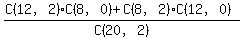
Or you can get the answer without using nCr, by looking at the probabilities of picking one marble at a time, as the other tutor does.